After a long time of not publishing anything and being passive about doing any writing in this blog, I am coming back for … however many articles I can. Today I want to talk about an underrated feature of AArch64 ISA which is often overlooked but used by compilers a lot. It’s just a good and short story on what made Arm even better and more “CISCy” when it comes down to conditional moves. The story of csinc deserves an article like this.
You probably heard of cmov
Traditionally, when you encounter conditional moves in literature, it is about x86 instruction cmov. It’s a nice feature and allows to accomplish better performance in low level optimization. Say, if you merge 2 arrays, you can compare numbers and choose the one depending on the value of compare instructions (more precisely, flags):
cmpl %r14d, %ebp   # compare which one is smaller, set CF
setbe %bl          # set CF to %bl if it's smaller
cmovbl %ebp, %r14d # move ebp into r14d if flag CF was set
If branches are unpredictable, for instance, you merge 2 arrays of random integers, conditional move instructions bring significant speed-ups against branchy version because of removing the branch misprediction penalty. A lot was written about this in the Lemire’s blog. Much engineering has been done on this including Agner Fog, cmov vs branch profile guided optimizations. Conditional move instructions are a huge domain of modern software, pretty much anything you run likely have them.
What about Arm?
AArch64 is no exception in this area and has some conditional move instructions as well. The immediate equivalent, if you Google it, is csel which is translated like conditional select. There is almost no difference to cmov except you specify directly which condition you want to check and destination register (in cmov the destination is unchanged if condition is not met). To my eye it is a bit more intuitive to read:
csel Xd, Xn, Xm, cond
When I was studying the structure of this instruction in the optimization guide, I noticed the family included different variations:
I was intrigued by the existence of some other forms as this involves more opportunities for the compilers and engineers to write software. For example, csinc Xd, Xa, Xb, cond (conditional select increase) means that if the condition holds, Xd = Xb + 1, otherwise Xd = Xa. For example, in merging 2 arrays, the line:
pos1 = (v1 <= v2) ? pos1 + 1 : pos1;
can be compiled into:
csinc X0, X0, X0, #condition_of_v1_less_equal_v2
where X0 is a register for pos1.
csneg, csinv are similar and represent conditional negations and inversions.
For example, clang recognizes this sequence, whereas GCC does not.
Interestingly enough, in compression! You might heard of Snappy, the old Google compression library which was surpassed by LZ4 many times. For x86, the difference in speed – even for the latest version of clang – is quite big. For example, on my server Intel Xeon 2.00GHz I have 2721MB/s of decompression for LZ4 and 2172MB/s for Snappy which is a 25% gap.
For Snappy to reach that level of decompression, engineers needed to write very subtle code to achieve cmov code generation:
This file contains hidden or bidirectional Unicode text that may be interpreted or compiled differently than what appears below. To review, open the file in an editor that reveals hidden Unicode characters.
Learn more about bidirectional Unicode characters
For Arm, csinc instruction was used because of the nature of the format:
Shortly, last 2 bits of the byte that opens the block have the instruction on what to do and which memory to copy: 00 copies len-1 data. With careful optimization of conditional moves, we can save on adding this +1 back through csinc:
On Google T2A instances I got 3048MB/s decompression for LZ4 and 2839MB/s which is only a 7% gap. If I enable LZ4_FAST_DEC_LOOP, I have 3233MB/s which still makes a 13% gap but not 25% as per x86 execution.
In conclusion, conditional select instructions for Arm deserve attention and awareness:
csel, csinc and others have same latency and throughput, meaning, they are as cheap as usual csel for almost all modern Arm processors including Apple M1, M2.
Compilers do recognize them (in my experience, clang did better than GCC, see above), no need to do anything special, just be aware that some formats might work better for Arm than for x86.
To sum up, contrary to the belief of CISC vs RISC debate about x86 and Arm ISA, the latter has surprising features of conditional instructions which are more flexible than the traditionally discussed ones.
TL;DR; We are changingstd::sort in LLVM’s libcxx. That’s a long story of what it took us to get there and all possible consequences, bugs you might encounter with examples from open source. We provide some benchmarks, perspective, why we did this in the first place and what it cost us with exciting ideas from Hyrum’s Law to reinforcement learning. All changes went into open source and thus I can freely talk about all of them.
This article is split into 3 parts, the first is history with all details of recent (and not so) past of sorting in C++ standard libraries. Second part is about what it takes to switch from one sorting algorithm to another with various bugs. The final one is about the implementation we have chosen with all optimizations we have done.
Chapter 1. History
Sorting algorithms have been extensively researched since the start of computer science.1 Specifically, people tried to optimize the number of comparisons on average, in the worst case, in certain cases like partially sorted data. There is even a sorting algorithm that is based on machine learning2 — it tries to predict the position where the elements should go with pretty impressive benchmarks! One thing is clear—sorting algorithms do evolve even now with better constant factors and reduced number of comparisons made.
In every programming language, sorting calls exist and it’s up to the library to decide which one to use, we’ll talk about different choices in languages later. There are still debates over which sorting is the best on Hackernews3, papers4, repos5.
As Donald Knuth said
It would be nice if only one or two of the sorting methods would dominate all of the others, regardless of application or the computer being used. But in fact, each method has its own peculiar virtues. […] Thus we find that nearly all of the algorithms deserve to be remembered, since there are some applications in which they turn out to be best.
— Donald Knuth, The Art Of Computer Programming, Volume 3
C++ history
std::sort has been in C++ since the invention of so-called “STL” by Alexander Stepanov9 and C++ standard overall got an interesting innovation back then called “complexity”. At the time the complexity was set to being comparisons on average. We know from Computer Science courses that quicksort is comparisons on average, right? This algorithm was first implemented in the original STL.
How was really the first std::sort implemented?
It used a simple quicksort with a median of 3 (median from (first, middle, last) elements). Once the recursion hits less than 16 elements, it bails out and at the end uses insertion sort as it is believed to work faster for small arrays.
You can see the last stage where it tries to “smooth out” inaccurate blocks of size 16.
A minor problem with quicksort
Well, that’s definitely true that quicksort has on average complexity, however, C++ STL may accept third parameter, called comp function:
This actually gives us an opportunity to self-modify the array, or, in other words, make decisions along the way the comp function is called, and introduce a worst time complexity on any data. The code below will make sense in a little while:
This file contains hidden or bidirectional Unicode text that may be interpreted or compiled differently than what appears below. To review, open the file in an editor that reveals hidden Unicode characters.
Learn more about bidirectional Unicode characters
If we consider any quick sort algorithm with the following semantics:
Find some pivot among elements (constant number)
Partition by pivot, recurse on both sides
“gas” value represents unknown, infinity, the value is set to the left element only when two unknown elements are compared, and if one element is gas, then it is always greater.
At the first step you pick some pivot among at most elements. While partitioning, all other elements will be to the right of the pivot.
At step you know the relation of at most elements and all elements will still be partitioned to the right. Take equals and you already have quadratic behavior.
If we run this code against the original STL10, we clearly are having a quadratic number of comparisons.
This file contains hidden or bidirectional Unicode text that may be interpreted or compiled differently than what appears below. To review, open the file in an editor that reveals hidden Unicode characters.
Learn more about bidirectional Unicode characters
No matter which randomization we are going to introduce, even quicksort implementation of std::sort is quadratic on average (with respect to arbitrary comparator) and implementation technically is not compliant.
The example above does not try to prove something and is quite artificial, even though there were some problems with the wording in the standard regarding “average” case.
Moving on with quadratic behavior
Quicksort worst case testing was first introduced by Douglas McIlroy11 in 1998 and called “Antiquicksort”. In the end it influenced the decision to move std::sort complexity being worst case rather than average which has been changed in the C++11 standard. The decision was partially made due to the fact there are lots of efficient worst case sorts out there as well.
Well, however there is more to the story.
Are modern C++ standard libraries actually compliant?
There are not so many places C++ standard specifies the wording “on average“. One more example is std::nth_element call.
What is std::nth_element?
You might guess it finds the nth element in the range. More specifically std::nth_element(first, nth, last, comp) is a partial sorting algorithm that rearranges elements in a range such that:
The element pointed at by nth is changed to whatever element would occur in that position if [first, last) were sorted.
All of the elements before this new nth element are less than or equal to the elements after the new nth element.
You can see that the complexity still states “on average“.
This decision was in place due to the existing quickselect12 algorithm. However, this algorithm is susceptible to the same trickery for both GNU and LLVM implementations.
For LLVM/clang version it’s obviously degrading to quadratic behavior, for GNU version for is around which are very close to reported numbers. If you read carefully the implementation13, you’ll see that the fallback algorithm uses heap select – by creating heap and extracting elements from it. And heap extraction is known to be logarithmic.
However, for finding nth element there are not so many worst case linear algorithms, one of them is median of medians16 which has a really bad constant. It took us around 20 years to find something really appropriate, thanks to Andrei Alexandrescu14 . My post on selection algorithms discussed that quite extensively but got too little attention in my humble opinion 🙂 (and it has an implementation from Andrei as well!). We found great speedups on real data for real SQL queries of type SELECT * from table ORDER BY x LIMIT N.
What happened to std::sort?
It started to use Introspective Sort, or, simply, introsort, upon too many levels of quicksort, more specifically , fall back to heap sort, worst case known algorithm. Even Wikipedia has all good references15 regarding introsort implementations.
Here is the worst case sorting introsort for GNU implementation:
LLVM history
When LLVM tried to build C++0x version of STL, Howard Hinnant made a presentation6 on how it all was going with the implementation. Back then we recognized some really interesting benchmarks and more and more benchmarked sorts on different data patterns.
Howard Hinnant’s slide on sorting in 2010
That gave us one interesting thought when we found this slide on what makes a sorting successful and efficient. Clearly not all data is random and some patterns happen in prod, how important is it to balance or recognize it?
For example even at Google as we use lots of protobufs, there are frequent calls to std::sort which come from the proto library7 which sorts all tags of fields presented in the message:
This file contains hidden or bidirectional Unicode text that may be interpreted or compiled differently than what appears below. To review, open the file in an editor that reveals hidden Unicode characters.
Learn more about bidirectional Unicode characters
This file contains hidden or bidirectional Unicode text that may be interpreted or compiled differently than what appears below. To review, open the file in an editor that reveals hidden Unicode characters.
Learn more about bidirectional Unicode characters
It makes a first quite important point: we need to recognize “almost sorted” patterns as they do happen. Obvious cases are ascending/descending, some easy mixes of those like pipes, and multiple consecutive increasing or decreasing runs. TL;DR; we did not do a very good job here but most modern algorithms do recognize quite obvious ones.
Condition 1 is a normalizer, condition 2 states that we should care only about comparisons and not elements, condition 3 shows that if you can sort a supersequence, you should be able to sort a subsequence in fewer amount of comparisons, condition 4 is an upper limit on sorted parts: you should be able to sort if you can sort and , condition 5 is a more general upper limit – you should be able to find position of in linear amount of comparisons.
There are many existing presortedness measures like
m01: 1 if not sorted, 0 if sorted. A pretty stupid one.
Block: Number of elements in a sequence that aren’t followed by the same element in the sorted sequence.
Mono: Minimum number of elements that must be removed from X to obtain a sorted subsequence, which corresponds to |X| minus the size of the longest non-decreasing subsequence of X.
Dis: Maximum distance determined by an inversion.
Runs: number of non-decreasing runs in X minus one.
Etc
Some presortedness measures are better than others, meaning if there exists an algorithm is optimal towards some measure (optimality means number of comparisons for all input behaves logarithmically on number on the inputs which have not bigger measure value: ), then it is also optimal towards another. And at this point, theory starts to differ much from reality. Theory found a nice “common” presortedness measure, it’s very complicated and out of scope for this article.
Unfortunately, among all measures above only Mono, Dis and Runs are linear time (others are and it’s an open question whether they have lower complexity). If you want to report some of these measures, you need to sample heavily or add extra to the sorting itself which is not great for performance. We could have done more work in that area but generally all we tried were microbenchmarks + several real world workloads.
Anyway, I guess you are tired of theory and let’s get to something more practical.
LLVM history continues
As LLVM libcxx was developed before C++11, the first version was also based on quicksort. What was the difference to the GNU sort?
The libcxx implementation handled a few particular cases specially. Collections of length 5 or less are sorted using special handwritten comparison based sortings.
This file contains hidden or bidirectional Unicode text that may be interpreted or compiled differently than what appears below. To review, open the file in an editor that reveals hidden Unicode characters.
Learn more about bidirectional Unicode characters
This file contains hidden or bidirectional Unicode text that may be interpreted or compiled differently than what appears below. To review, open the file in an editor that reveals hidden Unicode characters.
Learn more about bidirectional Unicode characters
Depending on the data type being sorted, collections of lengths up to 30 are sorted using insertion sort. Trivial types are easy to swap and assembly is quite good for them.
There is a special handling case for collections with most items being equal and for collections that are almost sorted. It tries to use insertion sort upon the limit of 8 transpositions: if during the outer loop we see more than 8 pair elements where , we bail out to recursion, otherwise we sort it and don’t go there. That’s really great for almost sorted patterns.
This file contains hidden or bidirectional Unicode text that may be interpreted or compiled differently than what appears below. To review, open the file in an editor that reveals hidden Unicode characters.
Learn more about bidirectional Unicode characters
However, if you look at ascending inputs, you can see libstdcxx does lots of unnecessary work compared to libcxx sort which matters in practice. First is literally running 4.5 times faster!
libcxx on ascending
libstdcxx on ascending
Last distinction was that the median of 5 was chosen when the number of elements in a quicksort partition is more than 1000. No more differences, for me the biggest impact of this sort is in trying to identify common patterns which is not cheap but gets lots of benefits for real world cases.
When we changed libstdcxx to libcxx at Google, we saw significant improvements (dozens of percent) spent in std::sort. From then, the algorithm hasn’t been changed, and the usage has been growing.
Quadratic problem
Given LLVM libcxx was developed for C++03, the first implementation targeted on average case we talked about earlier. That has been addressed several times in the past, in 2014, 2017, 201817, 18.
In the end we managed to submit an improvement same as GNU library has with introsort. We add an additional parameter to the algorithm that indicates the maximum depth of the recursion the algorithm can go, then the remaining sequence on that path is sorted using heapsort. The number of partitions allowed is set to . Since heapsort’s worst case time complexity is , the modified algorithm also has a worst case time complexity of . This change19 has been committed to the LLVM trunk and released with LLVM 14.
This file contains hidden or bidirectional Unicode text that may be interpreted or compiled differently than what appears below. To review, open the file in an editor that reveals hidden Unicode characters.
Learn more about bidirectional Unicode characters
How many real world cases got there into heap sort?
We also were curious how much performance went into deep levels of quicksort and confirmed that one in several thousand of all std::sort calls got into the fallback heapsort.
That was slightly unusual to discover. It also did not show any statistically significant performance improvements, i.e. no obvious or significant quadratic improvements have been found. Quicksort is really working ok on real world data, however, this algorithm can be exploitable.
Chapter 2. Changing sorting is easy, isn’t it?
At first it looks easy to just change the implementation and win resources: sorting has order and, for example, if you sort integers, the API does not care about the implementation; the range should be just ordered correctly.
However, the C++ API can take compare functions, which may be for simplicity lambda functions. We will call them “comparators.” These can break our assumptions about sorting being deterministic in several ways. Sometimes I refer to this problem a.k.a. “ties can be resolved differently”.
This file contains hidden or bidirectional Unicode text that may be interpreted or compiled differently than what appears below. To review, open the file in an editor that reveals hidden Unicode characters.
Learn more about bidirectional Unicode characters
This file contains hidden or bidirectional Unicode text that may be interpreted or compiled differently than what appears below. To review, open the file in an editor that reveals hidden Unicode characters.
Learn more about bidirectional Unicode characters
And we know that users like to write golden tests with queries of that sort. Even though nobody guarantees the order of equal elements, users do depend on that behavior as it might be buried down in code they have never heard of. That’s a classic example of Hyrum’s Law
With a sufficient number of users of an API,
it does not matter what you promise in the contract:
all observable behaviors of your system
will be depended on by somebody.
Hyrum Wright
Golden tests can be confusing if the diff is too big: are we breaking something or is the test too brittle to show anything useful to us? Golden tests are not a typical unit test because they don’t enforce any behavior. They simply let you know that the output of the service changed. There is no contract about the meaning of these changes; it is entirely up to the user to do whatever they want with this information.
When we tried to find all such cases, we understood it made the migration almost impossible to automate — how did we know these changes were the ones that the users wanted? In the end we learned a pretty harsh lesson that even slight changes in how we use primitives lead us to problems with goldens. It’s better if you use unit tests instead of golden ones or pay more attention to determinism of the code written.
Actually, about finding all Hyrum’s Law cases.
How to find all equal elements dependencies?
As equal elements are mostly indistinguishable during the compare functions (we found only a small handful of examples of comparators doing changes to array along the way), it is enough to randomize the range before the actual call to std::sort. You can figure out the probabilities and prove it is enough on your own.
We decided to submit such functionality into LLVM under debug mode20 for calls std::sort, std::nth_element, std::partial_sort.
This file contains hidden or bidirectional Unicode text that may be interpreted or compiled differently than what appears below. To review, open the file in an editor that reveals hidden Unicode characters.
Learn more about bidirectional Unicode characters
We used ASLR (address space layout randomization)21 technique for seeding the random number generator, meaning static variables will be in random addresses upon the start of the program and we can use it as a seed. This provides the same stability guarantee within a run but not through different runs, for example, for tests to become flaky and eventually be seen as broken. For platforms which do not support ASLR, the seed is fixed during build. Using other techniques from header <random> was not possible as header <algorithm> recursively depended on <random> and in such a low level library, we implemented a very simple linear generator.
This file contains hidden or bidirectional Unicode text that may be interpreted or compiled differently than what appears below. To review, open the file in an editor that reveals hidden Unicode characters.
Learn more about bidirectional Unicode characters
This randomization was enabled in a debug build mode as performance penalty might be significant for shuffling for all cases.
Partial vs nth danger
Also if you look closely at the randomization changes above, you may notice some difference between std::nth_element and std::partial_sort. That can be misleading.
std::partial_sort and std::nth_element have a difference in the meaning of their parameters that is easy to get confused. Both take 3 iterators:
begin – the beginning of the range
nth or middle – the meaning (and name) of this parameter differs between these functions
end – the end of the range
For std::partial_sort, the middle parameter is called middle, and points right after the part of the range that should end up sorted. That means you have no idea which element middle will point to – you only know that it will be one of the elements that didn’t need to be sorted.
For std::nth_element, this middle parameter is nth. It points to the only element that will be sorted. For all of the elements in [begin, nth) you only know that they’ll be less than or equal to *nth, but you don’t know what order they’ll be in.
That means that if you want to find the 10th smallest element of a container, you have to call these functions a bit differently:
This file contains hidden or bidirectional Unicode text that may be interpreted or compiled differently than what appears below. To review, open the file in an editor that reveals hidden Unicode characters.
Learn more about bidirectional Unicode characters
In the end, after dozens of runs of all tests at Google and with the help of a strong prevailing wind of randomness, we measured a couple of thousands of tests to be dependent on the stability of sorting and selection algorithms. As we also planned on updating sorting algorithms, this effort helped doing it gradually and sustainably.
All in all, it took us around a year to fix all of them.
Which failures will you probably discover?
Goldens
First of all, we, of course, discovered numerous failures regarding golden tests described above, that’s inevitable. From open source, you can try to look at ClickHouse22, 23, they also decided to introduce randomness described above.
Typical golden test updates
Most changes will look like this by adjusting the right ordering and updating golden tests.
Unfortunately, golden tests might be quite sensitive to production workloads, for example, during streaming engine rollout — what if some instances produce slightly different results for the same shard? Or what if some compression algorithm by accident uses std::sort and compares the checksum from another service which hasn’t updated its implementation? That might cause checksum mismatch, higher error rate, users suffering and even data loss, and you cannot easily swap the algorithm right away as it can break production workloads in unusual ways. Hyrum’s Law at its best and worst. For example, we needed to inject in a couple of places old implementations to allow teams to migrate.
Oh, crap, determinism
Some other changes might require a transition from std::sort to std::stable_sort if determinism is required. We recommend writing a comment on why this is important as stable_sort guarantees that equal elements will be in the same order as before the sort.
Side note: defaults in other languages are different and that’s probably good
In many languages24, including Python, Java, Rust, sort() is stable by default and, if being honest, that’s a much better engineering decision, in my opinion. For example, Rust has .sort_unstable() which does not have stability guarantees but explicitly tells what it does. However, C++ has a different priority, or, you may say, direction, i.e. usages of something should not do more than requested (a.k.a “You don’t pay for what you don’t use“). From our benchmarks std::stable_sort was 10-15% slower than std::sort, and it allocated linear memory. For C++ code that was quite critical given performance benefits. I like to think sometimes that Rust assumes more restrictive defaults with possibilities to relax them whereas C++ assumes less restrictive defaults with possibilities to tighten them.
Logical Bugs
We found several places where users invoked undefined behavior or made inefficiencies. Let’s get them from less to more important.
Sorting of binary data
If you compare by a boolean variable, for example, partition data by existence of something, it’s very tempting to write std::sort call.
This file contains hidden or bidirectional Unicode text that may be interpreted or compiled differently than what appears below. To review, open the file in an editor that reveals hidden Unicode characters.
Learn more about bidirectional Unicode characters
However, for compare functions that compare only by boolean variables, we have much faster linear algorithms, named std::partition and for stable version, std::stable_partition.
This file contains hidden or bidirectional Unicode text that may be interpreted or compiled differently than what appears below. To review, open the file in an editor that reveals hidden Unicode characters.
Learn more about bidirectional Unicode characters
Even though modern algorithms do a good job in detection of cardinality, try to prefer std::partition at least for readability issues.
Sorting more than needed
We saw a pattern of sort+resize a lot.
This file contains hidden or bidirectional Unicode text that may be interpreted or compiled differently than what appears below. To review, open the file in an editor that reveals hidden Unicode characters.
Learn more about bidirectional Unicode characters
You can work out from the code above that although each element must be inspected, sorting the whole of ‘vector’ (beyond the -th element) is not necessary. The compiler likely cannot optimize it away.
This file contains hidden or bidirectional Unicode text that may be interpreted or compiled differently than what appears below. To review, open the file in an editor that reveals hidden Unicode characters.
Learn more about bidirectional Unicode characters
Unfortunately, there is no stable std::partial_sort analogue, so fix a comparator if the determinism is required.
C++ is hard
If you have a mismatched type in a comparator, C++ will not warn you even with -Weverything. In the picture below zero warnings have been produced when sorting a vector of floats with std::greater<int> comparator.
Not following strict weak ordering
When you call any of the ordering functions in C++ including std::sort, compare functions much comply with the strict weak ordering which formally means the following:
Irreflexivity: is false
Asymmetry: and cannot be both true
Transitivity: and imply
Transitivity of incomparability: and imply , where means and are both false.
All these conditions make sense and algorithms actually use all those for optimization purposes. First 3 conditions set strict partial order, the 4th one is introducing equivalence relations on incomparable elements.
As you might imagine, we faced the violation of all conditions. In order to demonstrate those, I will post screenshots below where I found them through Github codesearch (https://cs.github.com). I promise I haven’t tried much to find bugs. The biggest emphasis is that violations do happen. After them we will discuss how they can be exploited
Violation of irreflexivity and asymmetry
This is a slideshow, look through it.
All of them violate irreflexivity, comp(x, x) returns true. You may say this might not be used in practice, however, we learned a tough lesson that even testing does not always help.
30 vs 31 elements. Happy execution vs SIGSEGV
You may remember that up to 30 elements for trivial types (and 6 for non-trivial), LLVM/libcxx sort uses insertion sort and after that it bails out to quicksort. Well, if you submit a comparator where conditions for irreflexivity or asymmetry are not met, you will find that with 31 elements the program might get into segfault whereas with 30 elements it works just fine. Consider this example, we want to move all negative elements to the right and sort all positive, same as some examples above.
We saw users writing tests for small ranges, however, when the number of elements grows, std::sort can result in SIGSEGV, and this may slip during testing, and be an interesting attack vector to kill the program.
This is used in the implementation of libcxx to wait for some condition to be false knowing we will at some point compare two equal elements:
This file contains hidden or bidirectional Unicode text that may be interpreted or compiled differently than what appears below. To review, open the file in an editor that reveals hidden Unicode characters.
Learn more about bidirectional Unicode characters
You can construct an example where the 4 condition is violated
The worst that can happen in that case with the current implementation that the elements would not be sorted (not segfaults, although this needs a proof but the article is already too big for that), check out:
And again, if you use fewer than 7 elements, insertion sort is used, and you will not construct a counter-example where std::is_sorted is not working. Even though, on paper this is undefined behavior, this is very hard to detect by sanitizers or tests, and in reality it passes simple cases.
Honestly, this snippet can be as simple as:
This file contains hidden or bidirectional Unicode text that may be interpreted or compiled differently than what appears below. To review, open the file in an editor that reveals hidden Unicode characters.
Learn more about bidirectional Unicode characters
Why? As doubles/floats can be NaN which means x < NaN and NaN < x are both false and that means x is equivalent to NaN thus for every finite x we have x == NaN but clearly x == NaN and y == NaN does not imply x == y.
So, if you have NaNs in the vector, calling std::sort on paper invokes undefined behavior. This is a part of the problem which was described in
Wait, but finding strict weak ordering violations takes cubic time
In order to detect strict weak ordering violations, you need to check all triples of elements which takes time. Even though with the existence of algorithms (this is for another post), this takes much more time than and likely cannot be used even in debug mode as programs will not finish for sorting a million elements in reasonable time.
And we did what most engineers would do. We decided after randomization to check triples and fixed or reported all bugs. Worked like a charm 🙂 . This hasn’t been submitted to LLVM yet as I could not find time to do that properly.
std::nth_element bug to randomization ratio is the highest. Here is why
Even though std::sort is used the most and found most failing test cases, we found that randomization for std::nth_element and std::partial_sort found more logical bugs per failing test case. I did a very simple codesearch query finding two close calls of std::nth_element and immediately found incorrect usages. Try to identify bugs on your own at first (you can find all of them in25):
All of them follow the same pattern of ignoring the results from the first nth_element call. The visualization for the bug can be seen in the picture:
And yes, this happens often enough, I didn’t even try to find many bugs, this was a 10 minutes skim through the github codesearch results. Fixes are trivial, access the nth element only after the call being made. Be careful.
How can you find bad sorting calls among hundreds of places in your codebase?
Users even in small repositories call std::sort in dozens/hundreds or even thousands different places, how can you find which sorting call introduces bad behavior? Well, sometimes it’s obvious, sometimes it’s definitely not and exploration is another question which greatly simplifies the debugging process.
We used inline variables26 (or sometimes compiler people call them weak symbols) in C++ which can be declared in headers and set from anywhere without linkage errors.
This file contains hidden or bidirectional Unicode text that may be interpreted or compiled differently than what appears below. To review, open the file in an editor that reveals hidden Unicode characters.
Learn more about bidirectional Unicode characters
This helped to find all stacktraces of std::sort calls and do some statistical analysis on where they come from. This still required a person to look at but greatly simplified the debugging experience.
A very small danger note
If the function backtrace_dumper uses std::sort somehow, then you might get into an infinite recursion. This method didn’t work from the first run as at Google we use allocator TCMalloc and it uses std::sort.
The same happened with absl::Mutex. These were funny hours finding out why unrelated tests failed 🙂
Also note that backtrace_dumper is likely needed to be thread safe.
Automating process by a small margin
Sometimes what you can do is the following:
Find all std::sort calls through this backtrace finder
Replace one by one with std::stable_sort
If tests become green, point to the user that this call is likely a culprit
Maybe suggest replacing it with std::stable_sort
Accepting a patch is sometimes easier than delegating to the team/person to fix it on their own
If none found, send a bug/look manually
This speeded up the process, and some teams accepted std::stable_sort understanding performance penalties, others realized that something was wrong and asked for a different fix.
Chapter 3. Which sorting are we replacing with?
In a way, that matters the least and does not require so much attention and effort from multiple people at the same time. If anybody decides to change the implementation, with the randomization above, it is easier to be prepared, switch and enjoy the savings (alongside with the benefits of mitigating serious bugs) right away. But our initial goal of this project was to provide better performance so we will talk a little about it.
I also want to admit that the debates around which sorting is the fastest are likely never going to stop and nonetheless it is important to move the needle towards greater algorithms. I am not going to claim the choice we proceed with is the best, it just significantly improves the status quo with several fascinating ideas.
A side note on distribution
We found that both cases are important to optimize, from sorting integers where comparisons are very cheap to extremely heavy where compare functions are even doing some codec decompression and thus are quite expensive. And as we said, it is quite important to figure out some patterns.
Branch (mis)predictions for cheap comparisons
This file contains hidden or bidirectional Unicode text that may be interpreted or compiled differently than what appears below. To review, open the file in an editor that reveals hidden Unicode characters.
Learn more about bidirectional Unicode characters
In the current implementation, sorting executes a significant number of branch instructions while partitioning the input about the pivot. The branches are shown above where their results decide to continue looping or not. These branches are quite hard to predict especially in cases when pivot is chosen to be right in the middle (for example, in random arrays). The mispredicted branches cause the process pipeline to be flushed and generally are considered harmful for the execution. This was quite known and carefully analyzed28, 29. In a way, it is sometimes better to choose a skewed pivot to avoid this heavy loop.
In order to mitigate this, we use the technique described in BlockQuickSort28.
BlockQuickSort aims to avoid most branches by separating the data movement from the comparison operation. This is achieved by having two buffers of size B which store the comparison results (for example, you can choose B=64 and store just 64 bit integers), one for the left side and the other for the right side while traversing the chunks of size B. Unlike the implementation above, it does not introduce any branches and if you do it right, compiler generates good SIMD code with wide 16 or 32 byte pcmpgt/pand/por instructions for both SSE4.2 and AVX2 code.
Once we fill all buffers, we should swap them around the pivot. Luckily, all we need to do is find the indices for the elements to swap next. Since the buffers reside in registers, we use ctz (count trailing zeros, in x86 bsf (Bit Scan Forward) or tzcnt (introduced in BMI)), blsr (Reset Lowest Set Bit, introduced in BMI) instructions to find the indices for the elements, thus avoiding any branch instructions.
Benchmarks showed about 50% savings on sorting random permutations of integers. You can look at them in https://reviews.llvm.org/D122780
Heavy comparisons
As we removed the mispredicted branches, now it is more reasonable to get other heuristics, for example, the pivot choice.
This file contains hidden or bidirectional Unicode text that may be interpreted or compiled differently than what appears below. To review, open the file in an editor that reveals hidden Unicode characters.
Learn more about bidirectional Unicode characters
The intuition behind is that a good pivot decreases the number of comparisons but increases the number of branch mispredictions. If we fix the latter, we can try to do the former as well. The more elements for pivot we consider in random arrays, the fewer comparisons we are going to make in the end.
Other small optimizations include unguarded insertion sort for not leftmost ranges during the recursion (out of all ranges, there is only 1 leftmost per each level of recursion), they all give small but sustainable benefits.
These are all in line with the pdqsort3 implementation which was quite acclaimed as a choice of implementation in other languages as well. And we see around 20-30% improvements on random data without sacrificing much performance for almost sorted patterns.
Reinforcement learning for small sorts
Another submitted change got some innovations in assembly generation for small sorts including cmov (conditional move instructions). This is the change https://reviews.llvm.org/D118029. What happened?
You might remember sort4 and sort5 functions from the beginning of the post. They are branchy, however, there are other ways to sort elements: sorting networks. They are the networks which abstract devices built up of a fixed number of “wires”, carrying values, and comparator modules that connect pairs of wires, swapping the values on the wires if they are not in a desired order. Optimal sorting networks are networks that sort the array with the least amount of such compare-and-swap operations made. For 3 elements you need to compare-and-swap 3 times, 5 times for 4 elements and an optimal sorting network for 5 elements consists of 9 compare-and-swap operations.
Optimal networks for bigger values remain an open question but how to break the conjecture the optimal networks for 11 and 12 elements you can read an absolutely amazing blog post Proving 50-Year-Old Sorting Networks Optimal30 by Jannis Harder.
x86 and ARM assembly have instructions called cmov reg1, reg2 and csel reg1, reg2, flag which move or select registers upon the value of comparisons. You can use that extensively for compare-and-swap operations.
And in order to swap elements through cmov with , comparisons, you need to do the following things:
loads from pointers, stores to pointers
For each comparison cmp instruction, mov for temporary register, 2 cmovs for swapping. Together instructions.
Together we have:
Sort2 – 8 instructions (2 elements and 1 comparison)
Sort3 – 18 instructions (3 elements and 3 comparisons)
Sort4 – 28 instructions (4 elements and 5 comparisons)
Sort5 – 46 instructions (5 elements and 9 comparisons)
Exactly 18 instuctions for sort3 on 64 bit integers, 1 for the name and 1 return instructions
However, as you can see, from the review above, sort3 is written in a little different way, with one conditional swap and magic swap.
This file contains hidden or bidirectional Unicode text that may be interpreted or compiled differently than what appears below. To review, open the file in an editor that reveals hidden Unicode characters.
Learn more about bidirectional Unicode characters
And if we paste it to Godbolt, we will see that such code produces 1 instruction less. The 19th line from the left got to the 16th on the right and the 15th line on the left was erased completely.
I guess this is the reinforcement learning authors talk about in the patch. Generation helped to find an opportunity by finding that if in a triple (X, Y, Z) the last 2 elements (Y <= Z) are sorted, it can be better done in 7 instructions rather than 8.
Move Z into tmp.
Compare X and Z.
Conditionally move X into Z.
Conditionally move X into tmp
Move tmp into X.this was deleted
Compare tmp and Y.
Conditionally move Y into X.
Conditionally move tmp into Y.
For sorting 4 integers there is no optimal network with such a pair of comparisons but for sort 5 there can be up to 3 pairs. In the end, patch found how to save 1 instruction in each red circle below. They are exactly pairs of wires where 2 elements are already sorted .
In the end that helped to reduce the number of instructions per small cases from 18->17 when comparing 3 integers, 46->43 when comparing 5 integers. Then there comes a question: in order to minimize the number of instructions, we likely want to produce such networks with the most amount of such magic swaps, that’s an open and great question to think about.
Are they actually faster? Well, in 18->17 case it is not always like that because the removed mov is greatly pipelined. It is still less work for the processor frontend to decode the instruction but you are not likely to see anything in the benchmarks. For 46->43 the situation is the same.
LLVM review claimed to save around 2-3% for integer benchmarks but they all mostly come from the transition from branchy version to a branchless one. Instruction reduction does not help much but anyway is a good story how machine learning can help driving compiler optimizations in such primitives as sorting networks together with assembly generation. I highly recommend reading the patch for all C++ lovers, it has lots of lovely ideas and sophisticated discussions on how to make it right31.
Conclusion
How can you help?
There are many things that are not yet done. Here is by no means an exhaustive list of things you can help with:
In debug modes introduce randomization described above.
This can be done for the GNU library, Microsoft STL, other languages like Rust, D, etc.
Introduce strict weak ordering debug checks in all functions that require it.
std::sort, std::partial_sort, std::nth_element, std::min_element, std::max_element, std::stable_sort, others, in all C++ standard libraries. In all other languages like Rust, Java, Python, D, etc. As we said, checking at most 20 elements per call seems to be ok. You can also introduce sampling if needed.
In your C++ project try to introduce a debug mode which sets _LIBCPP_DEBUG to some level27.
Consider randomization for the APIs that can be relied on at least in testing/debug mode. Seeding the hash function differently for not relying on the order of iteration of hashtables. If the function requires to be only associative, try to accumulate results in different order, etc.
Fix worst case std::nth_element in all standard library implementations.
Optimize assembly generation for sorts (small, big, partitions) even further. As you can see, there is room for optimizations there as well!
Final thoughts
We started this process more than a year ago (of course, not full time), and the first primary goal was performance. However, it turned out to be a much more sophisticated issue. We found several hundred bugs (including pretty critical ones). In the end, we figured out a way to prevent bugs from happening in the future which will help us to adopt any correct implementation and, for example, see wins right away without being blocked by broken tests. We suggest if your codebase is huge, adopt the build flag from libcxx and prepare yourself for the migration. Most importantly, this effort produced a story on how to change even simplest things at scale, how to fight Hyrum’s Law, and I am glad to be a part of the effort to help open source learn from it.
Acknowledgements
Thanks to Nilay Vaish who pushed the changes for a new sort to LLVM, thanks to Louis Dionne, the maintainer of libcxx, who patiently accepted our changes. Thanks to Morwenn for outstanding work on sorting from which I learned a lot5. Thanks to Orson Peters and pdqsort which greatly improved the performance of modern in-memory sorting.
References
The famous textbook from Cormen and others Introduction to Algorithms devotes over 50 pages to sorting algorithms.
H. Mannila, “Measures of Presortedness and Optimal Sorting Algorithms,” in IEEE Transactions on Computers, vol. C-34, no. 4, pp. 318-325, April 1985, doi: 10.1109/TC.1985.5009382.
TCMalloc team recently published a paper on OSDI’21 about Google’s allocator internals, specifically on how huge pages are used. You can read the full paper here.
TL;DR. Google saved 2.4% of the memory fleet and increased the QPS performance of the most critical applications by 7.7%, an impressive result worth noting. Code is open sourced, you can find it on GitHub.
My experience with huge pages has never been a success, several years ago at my previous company I tried enabling them and got zero results, surprisingly, I believe Google also tried them and got nothing out of just huge pages. However, if you see zero performance with better packing opportunities, it is worth trying to pack allocations together on such pages and releasing to the OS complete ones. This is a finally successful approach with significant gains.
A hugepage-aware allocator helps with managing memory contiguity at the user level. The goal is to maximally pack allocations onto nearly-full hugepages, and conversely, to minimize the space used on empty (or emptier) hugepages, so that they can be returned to the OS as complete hugepages. This efficiently uses memory and interacts well with the kernel’s transparent hugepage support.
Section 2
The paper is heavily based on some structure of TCMalloc, you can find a probably slightly outdated design in that link but let’s just revise a couple of points.
Objects are segregated by size. First, TCMalloc partitions memory into spans, aligned to TCMalloc’s page size (in picture it is 25 KiB).
Sufficiently large allocations are fulfilled with a span containing only the allocated object. Other spans contain multiple smaller objects of the same size (a sizeclass). The “small” object size boundary is 256 KiB. Within this “small” threshold, allocation requests are rounded up to one of 100 sizeclasses. TCMalloc stores objects in a series of caches.
TCMalloc structure
The lowest one is per hyperthread cache which is tried first to satisfy the allocation (currently they are 256KiB) storing a list of free objects for each sizeclass (currently there are 86 or 172 of them which are defined here). When the local cache has no objects of the appropriate sizeclass to serve a request, then it goes to central and transfer caches which contain spans of those sizeclasses.
Some statistics
Most allocations are small: 55% of them are less than 8KB, 70% less than 1MB, 90% less than 10MB, other 10% grow linearly from 10MB to 10GB.
So most fight is going for small and middle sized allocations, up to several MB.
Temeraire
This technology (main contribution) replaces the pageheap with an ability to utilize 2MB hugepages. Paper tries to stick to several postulates
Total memory demand varies unpredictably with time, but not every allocation is released. Paper argues that both types of allocations are important and there is no skew in any — long lived and short lived ones are both critical.
Completely draining hugepages implies packing memory at hugepage granularity. Generating nearly empty hugepages implies densely packing the other hugepages.
Draining hugepages gives us new release decision points. Returning pages should be chosen wisely, if we return too often, that is costly, if we return too rare, that would lead to higher memory consumption.
Mistakes are costly, but work is not. Better decisions on placement and fragmentation are almost always better than additional work to make it right.
Then Temeraire introduces 4 different entities, HugeAllocator, HugeCache, HugeFiller and HugeRegion. And a couple of definitions: slack memory is a memory that remains unfulfilled in a huge page, backed memory is a memory which is allocated by the OS and in possession of a process and unbacked is returned to/unused in OS memory.
Allocation algorithm
HugeAllocator deals with all OS stuff, responsible for all unbacked hugepages. HugeCache stores backed, fully-empty hugepages. HugeFiller is responsible for all partially filled single hugepages. HugeRegion allocator is a separate entity when medium requests are fulfilled by HugeCache with a high ratio of slack memory. HugeCache with all its slack memory donate it to HugeFiller to fill smaller allocations.
Several words about all allocators.
HugeAllocator
HugeAllocator tracks mapped virtual memory. All OS mappings are made here. It stores hugepage-aligned unbacked ranges. The implementation tracks unused ranges with a treap.
HugeCache
The HugeCache tracks backed ranges of memory at full hugepage granularity. This thing is tracking all big allocations and should be responsible for releasing the pages (making from backed to unbacked). However, if you just allocate-deallocate in a loop, you need to compute some statistics because lots of memory is going to be held unused. Authors suggest calculating the demand of how much memory is requested in a 2 second window and returning to the OS if the cache size is bigger than the peaks of the demand. One note: from code I see that they try to have several pages in the cache anyway (10, if being precise), I believe this is important as weird cases on small allocations can happen and releasing everything might be costly, having something backed is a good thing.
At the same time it helps to avoid pathological cases of allocating/deallocating things a lot and be on the same total usage, for example, see for tensorflow.
HugeFiller
Most interesting part, most allocations end up here. This component solves the binpacking problem: the goal is to segment hugepages into some that are kept maximally full, and others that are empty or nearly so. Another goal is to minimize fragmentation within each hugepage, to make new requests more likely to be served. If the system needs a new K-page span and no free ranges of ≥ K pages are available, we require a hugepage from the HugeCache. This creates slack of (2MiB−K ∗ pagesize), wasting space.
Both priorities are satisfied by preserving hugepages with the longest free range, as longer free ranges must have fewer in-use blocks. We organize our hugepages into ranked lists correspondingly, leveraging per-hugepage statistics.
Section 4.4
Inside each hugepage, a bitmap of used pages is tracked (TCMalloc pages); to fill a request from some hugepage a best-fit search is done from that bitmap. Together with this bitmap, some statistics is stored:
The Longest free range (L). The number of contiguous pages (simple ones, not hugepages) not already allocated
Total number of allocations (A)
Hugepages with the lowest sufficient L and highest A are chosen to place the allocation. The intuition behind that is to avoid allocations from hugepages with very few allocations. Then the radioactive decay-type allocation model is used with logarithmic scale (because 150 allocations on a hugepage is the same as 200 and smaller numbers matter the most).
HugeRegion
HugeRegion helps allocations between HugeFiller and HugeCache. If we have requests of 1.1MiB then we have a slack of 0.9MiB which leads to high fragmentation. A HugeRegion is a large fixed-size allocation (currently 1 GiB) tracked at small-page granularity with the same kind of bitmaps used by individual hugepages in the HugeFiller. Instead of losing 0.9MiB per page, now it is lost per region.
Results
Decreased TLB misses
Overall, a point that stuck in my head is that “Gains were not driven by reduction in the cost of malloc.“, they came from speeding up user code. As an example, ads application showed 0.8% regression in TCMalloc itself but 3.5% improvement in QPS and 1.7% in latency. They also compare tens of other stuff but as you can guess, everything becomes better.
The best quote I found in this paper is probably not even a technical one but rather a methodological:
It is difficult to predict the best approach for a complex system a priori. Iteratively designing and improving a system is a commonly used technique. Military pilots coined the term “OODA (Observe, Orient, Decide, Act) loop” to measure a particular sense of reaction time: seeing incoming data, analyzing it, making choices, and acting on those choices (producing new data and continuing the loop). Shorter OODA loops are a tremendous tactical advantage to pilots and accelerate our productivity as well. Optimizing our own OODA loop–how quickly we could develop insight into a design choice, evaluate its effectiveness, and iterate towards better choices–was a crucial step in building TEMERAIRE.
Section 6
There is also the human side. Short OODA loops are candy. We really like candies and if some candy is taking too long, we go looking for another candy elsewhere.
Conclusion
Overall paper describes lots of ideas from allocators, how to build them, what should be considered as important and introduces finally a successful approach of supporting hugepages inside it with significant improvements which were mostly done by fast iterations rather than complex analysis and talent of ideas. Yet, there are still many other directions to try out like understanding immortal allocations, probably playing with the hardware, cold memory and further small and big optimizations, yet, this is a very well written and nicely engineered approach on how to deal with memory at Google’s scale.
A friend of mine nerd sniped me with a good story to investigate which kinda made me giggle and want to tell to the public some cool things happened to me during my experience with hashing and other stuff.
The story is simple and complex at the same time, I’d try to stick to a simple version with the links for those who do understand the underlying computations better.
A Cyclic Redundancy Check (CRC) is the remainder of binary division of a potentially long message, by a CRC polynomial. This technique is employed in network and storage applications due to its effectiveness at detecting errors. It has some good properties as linearity.
Speaking in mathematical language CRC is calculated in the following way:
where the polynomial defines the CRC algorithm and the symbol denotes carry-less multiplication. Most of the times the polynomial is irreducible, it just leads to fewer errors in some applications. CRC-32 is basically a CRC with of degree 32 over Galois Field GF(2). Nevermind, it still does not matter much, mostly for the context.
x86 processors for quite some time have instructions CLMUL which are responsible for multiplication in GF(2) and can be enabled with -mplcmul in your C/C++ compilers. They are useful, for example, in erasure coding to speed up the recovery from the parity parts. As CRC uses something similar to this, there are algorithms that speed up the CRC computation with such instructions.
The main and almost the only one source of knowledge how to do it properly with other SIMD magic is Fast CRC Computation for Generic Polynomials Using PCLMULQDQ Instruction from Intel which likely hasn’t been changed since 2009, it has lots of pictures and it is nice to read when you understand the maths. But even if you don’t, it has a well defined algorithm which you can implement and check with other naive approaches that it is correct.
When it tries to define the final result, it uses so called scary Barrett reduction which is basically the subtraction of the inverse times the value. Just some maths.
Still not so relevant though. But here comes the most interesting part. In the guide there are some constants for that reduction for gzip CRC. They are looking this way
Look at k6′ and u’
If we look closely, we would notice that k6′ and u’ are ending in 640 and 641 respectively. So far, so good, yet, in the Linux kernel the constants are slightly different, let me show you
It is stated to be written from the guide in the header, so they should be same. The constant is 0x1DB710641 vs 0x1DB710640 stated in the guide, the off by 1 but with the same 3 digits in the end as u’.
Two is that there’s also this line a little earlier on the same page: = 0x1DB710641 This number differs from only in the final bit: 0x41 vs 0x40. This isn’t coincidental. Calculating (in the Galois Field GF(2) space) means dividing (i.e. bitwise XOR-ing) a 33-bit polynomial (, with only one ‘on’ bit) by the 33-bit polynomial .
I thought for a while this is a legitimate bug. But wait a second, how can this be even possible given that CRC is used worldwide.
I decided that this is too good to be true to be a bug, even though the number is changed, I also tried 0x42 and the tests fail. After that I started looking at the code and managed to prove that this constant +-1 does not matter
Let’s look the snippet where this constant is used from zlib:
This file contains hidden or bidirectional Unicode text that may be interpreted or compiled differently than what appears below. To review, open the file in an editor that reveals hidden Unicode characters.
Learn more about bidirectional Unicode characters
Speaking about CLMUL instruction, it has the following signature __m128i _mm_clmulepi64_si128 (__m128i a, __m128i b, const int imm8), i.e. takes two 16 byte registers and mask and returns 16 byte register. The algorithm is the following
While executing the 15th line in gist x2 = _mm_clmulepi64_si128(x2, x0, 0x10); the mask imm8 takes the high 8 bytes in TEMP2 and thus the result isn’t changed, no need to worry here.
The most interesting part is the second _mm_clmulepi64_si128 with the third argument 0x00 which takes first 8 bytes from the operation in TEMP2. Actually the resulting values would be different but all we need to prove is that the bytes from 4 to 8 are the same because return happens with _mm_extract_epi32 which returns exactly uint32_t of that bytes (to be clear, the xor from x1 and x2 but if we prove bytes from 4 to 8 are the same for x2, it would be sufficient).
The bytes from 4 to 8 are only used in one loop in the operation:
TEMP2 is now our “magic” k6 value and TEMP1 is just some input. Note that when changing from 0x1DB710640 to 0x1DB710641 we only swap bit TEMP2[0]. Given it makes AND with all bits when i equals to j, the result would not change if and only if TEMP1[j] is zero for all j from 32 to 63.
And this turns out to be true because before the second CLMUL happens the following: x2 = _mm_and_si128(x2, x3);. And as you can see, x3 has bits zero from 32 to 63. And the returning result isn’t changed. What a coincidence! Given the conditions, if the last byte is changed to 0x42, only the highest bit can differ at the very most as it changes TEMP2[1].
For now I don’t know for 100% if it was made on purpose, to me looks like a human issue where the value was copy pasted and accidentally it worked. I wish during the interviews I also may miss any +-1 because of such bit magic 🙂
Bonus: speaking about CRC
This is not for the first time I face some weird bit magic issues with CRC, for example, look at the following code:
This file contains hidden or bidirectional Unicode text that may be interpreted or compiled differently than what appears below. To review, open the file in an editor that reveals hidden Unicode characters.
Learn more about bidirectional Unicode characters
It seeds CRC64 hash with FNV hash and the results are the same. Though the last byte of the 8 word strings are different. I faced it once in URL hashing and it was failing for urls with very short domain and path. The proof is left as an exercise to the reader, try it out, really, it is some good bit twiddling. More hashing is sometimes bad hashing, be careful 🙂
Thanks to Nigel Tao who first suspected an issue with the Linux kernel and described it in the wuffs repository. I think no one should do anything as it perfectly works or at the very most fix the constants to better match the guideline.
Today I present a big effort from my side to publish miniselect — generic C++ library to support multiple selection and partial sorting algorithms. It is already used in ClickHouse with huge performance benefits. Exact benchmarks and results will be later in this post and now let’s tell some stories about how it all arose. I publish this library under Boost License and any contributions are highly welcome.
It all started with sorting
While reading lots of articles, papers, and posts from Hacker News, I found it pretty funny each several months new “shiny”, “fastest”, “generic” sorting algorithms to come or remembered from old papers such as the recent paper on learned sorting, Kirkpatrick-Reisch sort or pdqsort. It is that we are essentially 65+ years into writing sorting algorithms, and we still find improvements. Shouldn’t sorting items be a “solved” problem by now? Unfortunately, not. New hardware features come, we find that sorting numbers can be actually done faster than best comparison time complexity and we still find improvements in sorting algorithms like avoiding branches in partitions and trying to find good pivots as pdqsort does. Also, there are many open questions in that area as “what is the minimum number of comparisons needed?”.
Huge competition is still going on in sorting algorithms and I believe we are not near the optimal sorting and learned sorting looks like the next step. But it uses the fundamental fact that no one expects sorting to be completed in a couple of passes and we can understand something about data during first array passes. We will understand why it matters later.
My favorite general sorting is pdqsort, it proves to be currently the best general sorting algorithm and it shows a significant boost over all standard sorts that are provided in C++. It is also used in Rust.
Selection and Partial Sorting
Nearly a couple of months ago I started thinking about a slightly different approach when it comes to sorting — partial sorting algorithms. It means that you don’t need to sort all elements but only find smallest and sort them. For example, it is widely used in SQL queries when you do ORDER BY LIMIT N and N is often small, from 1-10 to ideally couple of thousands, bigger values still happen but rare. And, oh god, how little engineering and theoretical research has been done there compared to full sorting algorithms. In fact, the question of specifically finding th order statistics when is small is open and no good solution is presented. Also, partial sorting is quite easy to obtain after that, you need to sort the first elements by some sorting algorithm to get optimal comparisons and we will look at only one example when it is not the case. Yes, there are a bunch of median algorithms that can be generalized to find the th smallest element. So, what are they? Yeah, you may know some of them but let’s revise, it is useful to know your enemies.
QuickSelect
This is almost the very first algorithm for finding the th smallest element, just do like QuickSort but don’t go recursively in two directions, that’s it. Pick middle or even random element and partition by this element, see in which of two parts is located, update the one of the borders, voila, after maximum of partitions you will find th smallest element. Good news that on average it takes comparisons if we pick random pivot. That is because if we define is the expected number of comparisons for finding th element in elements and , then during one stage we do comparisons and uniformly pick any pivot, then even if we pick the biggest part on each step
If assuming by induction that with an obvious induction base, we get
Bad news is that the worst case will still be if we are unfortunate and always pick the biggest element as a pivot, thus partitioning .
In that sense that algorithm provides lots of pivot “strategies” that are used nowadays, for example, picking pivot as a element of the array or picking pivot from 3 random elements . Or do like std::nth_element from libcxx — choose the middle out out of .
I decided to visualize all algorithms I am going to talk about today, so quickselect with a median of 3 strategy on random input looks something like this:
nth_element in libcxx, median of 3 strategies
And random pivot out of 3 elements works similar
Finding median in median of 3 random algorithm
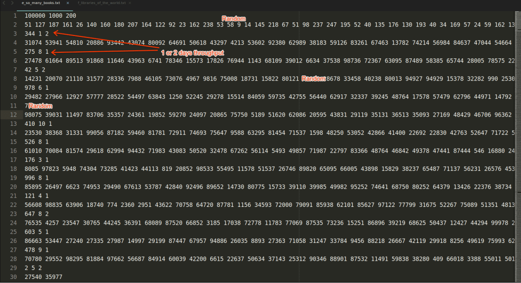
For a strategy like libcxx (C++ llvm standard library) does, there are quadratic counterexamples that are pretty easy to detect, such patterns also appear in real data. The counterexample looks like that:
This file contains hidden or bidirectional Unicode text that may be interpreted or compiled differently than what appears below. To review, open the file in an editor that reveals hidden Unicode characters.
Learn more about bidirectional Unicode characters
For a long time, computer scientists thought that it is impossible to find medians in worst-case linear time, however, Blum, Floyd, Pratt, Rivest, Tarjan came up with BFPRT algorithm or like sometimes it is called, median of medians algorithm.
Median of medians algorithm: Given array of size and integer ,
Group the array into groups of size 5 and find the median of each group. (For simplicity, we will ignore integrality issues.)
Recursively, find the true median of the medians. Call this .
Use as a pivot to partition the array.
Recurse on the appropriate piece.
When we find the median of groups, at least of them have at least 3 out of 5 elements that are smaller or equal than , that said the biggest out of 2 partitioned chunks have size and we have the reccurence
If we appropriately build the recurse tree we will see that
This is the geometric series with which gives us the result .
Actually, this constant 10 is really big. For example, if we look a bit closer, is at least 1 because we need to partition the array, then finding median out of 5 elements cannot be done in less than 6 comparisons (can be proven by only brute-forcing) and in 6 comparisons it can be done in the following way
Use three comparisons and shuffle around the numbers so that , and .
If , then the problem is fairly easy. If , the median value is the smaller of and . If not, the median value is the smaller of and .
So . If , then the solution is the smaller of and . Otherwise, the solution is the smaller of and .
So that maximum can be and it gives us the upper bound comparisons which looks like it can be achieved. Some other tricks can be done in place to achieve a bit lower constants like (for example, sorting arrays of 5 and comparing less afterwards). In practice, the constant is really big and you can see it from the following demonstration which was even fastened because it took quite a few seconds:
Median of medians for random input
HeapSelect
Another approach to finding th element is to create a heap on an array of size and push other elements into this heap. C++ std::partial_sort works that way (with additional heap sorting of the first heap). It shows good results for very small and random/ascending arrays, however starts to significantly degrade with growing and becomes impractical. Best case , worst , average .
std::partial_sort, two stages, first HeapSelect then heap sort of the first half, accelerated for speed
IntroSelect
As the previous algorithm is not very much practical and QuickSelect is really good on average, in 1997 “Introspective Sorting and Selection Algorithms” from David Musser came out with a sorting algorithm called “IntroSelect”.
IntroSelect works by optimistically starting out with QuickSelect and only switching to MedianOfMedians if it recurses too many times without making sufficient progress. Simply limiting the recursion to constant depth is not good enough, since this would make the algorithm switch on all sufficiently large arrays. Musser discusses a couple of simple approaches:
Keep track of the list of sizes of the subpartitions processed so far. If at any point recursive calls have been made without halving the list size, for some small positive , switch to the worst-case linear algorithm.
Sum the size of all partitions generated so far. If this exceeds the list size times some small positive constant , switch to the worst-case linear algorithm.
This algorithm came into libstdcxx and guess which strategy was chosen? Correct, none of them. Instead, they try QuickSelect steps and if not successful, fallback to HeapSelect algorithm. So, worst case , average
std::nth_element in libstdcxx, “IntroSelect”
PDQSelect
Now that most of the known algorithms come to an end 😈, we can start looking into something special and extraordinary. And the first one to look at is pdqselect which comes pretty straightforward from pdqsort, the algorithm is basically QuickSelect but with some interesting ideas on how to choose an appropriate pivot:
If there are elements, use insertion sort to partition or even sort them. As insertion sort is really fast for a small amount of elements, it is reasonable
If it is more, choose — pivot:
If there are less or equal than 128 elements, choose pseudomedian (or “ninther”, or median of medians which are all them same) of the following 3 groups:
begin, mid, end
begin + 1, mid – 1, end – 1
begin + 2, mid + 1, end – 2
If there are more than 128 elements, choose median of 3 from begin, mid, end
Partition the array by the chosen pivot with avoiding branches:
The partition is called bad if it splits less than elements
If the total number of bad partitions exceeds , use std::nth_element or any other fallback algorithm and return
Otherwise, try to defeat some patterns in the partition by (sizes are l_size and r_size respectively):
Swapping begin, begin + l_size / 4
Swapping p – 1 and p – l_size / 4
And if the number of elements is more than 128
begin + 1, begin + l_size / 4 + 1
begin + 2, begin + l_size / 4 + 2
p – 2, p – l_size / 4 + 1
p – 3, p – l_size / 4 + 2
Do the same with the right partition
Choose the right partition part and repeat like in QuickSelect
pdqselect on random input
Median Of Ninthers or Alexandrescu algorithm
For a long time, there were no practical improvements in finding th element, and only in 2017 very well recognized among C++ community Andrei Alexandrescu published a paper on Fast Deterministic Selection where worst case median algorithm becomes practical and can be used in real code.
There are 2 key ideas:
We now find the pseudomedian (or ninther, or median of medians which are all the same) of 9 elements as it was done similarly in pdqsort. Use that partition when
Introduce MedianOfMinima for . MedianOfMedians computes medians of small groups and takes their median to find a pivot approximating the median of the array. In this case, we pursue an order statistic skewed to the left, so instead of the median of each group, we compute its minimum; then, we obtain the pivot by computing the median of those groupwise minima.
is not chosen arbitrarily because in order to preserve the linearity of the algorithm we need to make sure that while recursing on elements we partition more than elements and thus . MedianOfMaxima is done the same way and for . The resulting algorithm turns out to be the following
Turns out it is a better algorithm than all above (except it did not know about pdqselect) and shows good results. My advice that if you need a deterministic worst-case linear algorithm this one is the best (we will talk about a couple of more randomized algorithms later).
QuickSelect adaptive on random data
Small k
All these algorithms are good and linear but they require lots of comparisons, like, minimum for all . However, I know a good algorithm for which requires only comparisons (I am also not going to prove it is minimal but it is). Let’s quickly revise how it works.
For finding a minimum you just compare linearly the winner with all others and basically the second place can be anyone who lost to the winner, so we need to compare them within each other. Unfortunately, the winner may have won linear number of others and we will not get the desired amount of comparisons. To mitigate this, we need to make a knockout tournament where the winner only plays games like that:
And all we need to do next is to compare all losers to the winner
And any of them can be the second. And we use only comparisons for that.
What can we do to find the third and other elements? Possibly not optimal in comparison count but at least not so bad can follow the strategy:
First set up a binary tree for a knockout tournament on items. (This takes comparisons.) The largest item is greater than others, so it can’t be th largest. Replace it, where it appears at an external node of the tree, by one of the elements held in reserve, and find the largest element of the resulting ; this requires at most comparisons because we need to recompute only one path in the tree. Repeat this operation times in all, for each element held in reserve.
It will give us the estimation of comparisons. Assume you need to find top 10 out of millions of long strings and this might be a good solution to this instead of comparing at least times. However, it requires additional memory to remember the path of the winner and I currently do not know how to remove it thus making the algorithm impractical because of allocations or additional level of indirections.
At that time my knowledge of selection algorithms ended and I decided to address one known guy.
You know him
In The Art of Computer Programming, Volume 3, Sorting and Searching I read almost 100-150 pages in order to understand what the world knows about minimal comparison sorting and selection algorithms and found a pretty interesting one called Floyd-Rivest algorithm. Actually, even Alexandrescu paper cites it but in an unusual way:
Floyd-Rivest algorithm
This algorithm is essentially the following
The general steps are:
Select a small random sample of size from the array.
From , recursively select two elements, and , such that (essentially they take and ). These two elements will be the pivots for the partition and are expected to contain theth smallest element of the entire list between them.
Using and , partition into three sets (less, more and between).
Partition the remaining elements inthe array by comparing them to u or v and placing them into the appropriate set. If is smaller than half the number of the elements in the array, then the remaining elements should be compared to first and then only to if they are smaller than . Otherwise, the remaining elements should be compared to first and only to if they are greater than .
Apply the algorithm recursively to the appropriate set to select the th smallest in the array.
Then in 2004 it was proven that this method (slighly modified in bound selection) will have comparisons with probability at least (and the constant in the power can be tuned).
This algorithm tries to find the appropriate subsamples and proves that the th element will be there with high probability.
Floyd-Rivest median on random dataFloyd-Rivest k=n/10 order statistics
Yet the worst case of the algorithm is still but it tries to optimize the minimum amount of comparisons on average case, not the worst case.
For small it is really good as it only used comparisons which is significantly better than all “at least comparisons” algorithms and even for median it is which is significantly better.
What it resulted in
So I decided to code all these algorithms with the C++ standard API and to test against each other and possibly submit to something performance heavy as DBMS for ORDER BY LIMIT N clauses.
I ended up doing miniselect library. For now, it is header-only but I don’t guarantee that in the future, it contains almost all algorithms except the tournament one which is very hard to do in the general case.
I tested on Intel(R) Core(TM) i5-4200H CPU @ 2.80GHz (yeah, a bit old, sorry). We are going to find median and 1000th elements out of and arrays. Benchmark data:
Ascending
Descending
Median3Killer which I described above
PipeOrgan: half of the values are ascending, the other half is descending
PushFront: ascending but the smallest element added to the end
PushMiddle: ascending but the middle element added to the end
As you see, Floyd-Rivest outperforms in time all other algorithms and even Alexandrescu in most of the cases. One downside is that Floyd-Rivest performs worse on data where there are many equal elements, that is expected and probably can be fixed as it is pointed out in Kiwiel’s paper.
As you see, most of the queries have ORDER BY LIMIT N. Topmost queries were significantly optimized because std::partial_sort works worst when the data is descending, real-world usage as you can see in string_sort benchmarks was optimized by 10-15%. Also, there were many queries that have been optimized by 5% where sorting is not the bottleneck but still, it is nice. It ended up with a 2.5% overall performance boost across all queries.
Other algorithms showed worse performance and you can see it from the benchmarks above. So, now Floyd-Rivest is used in production, and for a good reason. But, of course, it does not diminish the results of Mr. Alexandrescu and his contributions are very valuable when it comes to determinism and worst case.
Library
I publish miniselect under Boost License for everybody to use and adjust to the projects. I spent several days in the last week trying to make it work everywhere (except Windows for now but it should be good). We support C++11 and further with GCC 7+ and Clang 6+. We carefully test the algorithms for standard compliance, with fuzzing, sanitizers, etc. Fuzzing managed to find bugs that I thought only at the last moment so it really helps.
If you want to use it, please read the API but it should be an easy sed/perl/regex replacement with zero issues except for the ties between elements might resolve in a different way, however, C++ standard says it is ok and you should not rely on that.
Any contributions and other algorithms that I might miss are highly welcome, I intend to get this library as a reference to many implementations of selection algorithms so that the users can try and choose the best options for them. (Should I do the same for sorting algorithms?)
Conclusion
This was a long story of me trying to find the solutions to the problems that were puzzling me for the past month or so. I probably read 300+ pages of math/algorithms/discussions/forums to finally find everything that the world knows about it and to make it work for real-world applications with huge performance benefits. I think I can come up with something better in a long term after researching this stuff for a while longer but I will let you know in this blog if anything arises 🙂
References I find useful (together with zero mentions in the post)
Selection Algorithms with Small Groups where the Median of Medians algorithms are a little bit twisted for groups of size 3 and 4 with linear time worst-case guarantee
Today I present miniselect — generic C++ library for various selection algorithms https://t.co/NAJmqMOE8a. Aaand post about my efforts and research in that area https://t.co/YrNgZshrAJ. Many insights and gifs are included!
Hello everyone, today we are going to talk about C++ performance. Again, another “usual” perf blog as you may think. I promise to give really practical advice and don’t get bullshitty (okay, a little bit) talks about how C++ is performant. We are gonna roast the compilers and think about what we should do about it (or should we?). Let’s do a bit of fact-checking:
Fact #1. Compilers are smarter than the programmers
Resolution: it’s exaggerated
Of course, we do have really awesome compiler infrastructure as GNU or LLVM, they are doing a massively great job in optimizing programs. Hundreds of PhDs were wasted done on researching that and what the community achieved is flabbergastingly.
However, the problem of finding the optimal program is undecidable, and nothing we can do about it. Even small cases of invariant loads are not simplified, after looking at the examples below it seems that compilers cannot do anything useful:
None of the expressions were optimized to one load but they clearly should be. I was always thinking that compilers should find all possible invariants in the code and simplify the constructions to minimize the execution cost.
Compilers cannot understand the complex properties of the ranges being sorted or increasing which can help understanding more structures. Actually, that’s because of the compilation times — understanding the sorted property is rarely used and is not so easy to check or make the programmers annotate.
Also, of course, no compiler will optimize your quadratic sort into a O(n log n) sort because it is too much for them to understand what you really want and other factors can play a role — for example, the stability of sorting which affects the order of equal elements, etc.
Fact #2. C/C++ produces really fast code
Resolution: false
I don’t agree that C/C++ itself provides the best performance in the world, the only thing I am convinced in: C/C++ provides you the control over your performance. When you really really want to find the last nanoseconds in your program, C++ is a great tool to achieve this, for example, you can look at my blog entry on how I managed to put 16 byte atomics in the Abseil, doing it in other languages require much more time and not that expressive.
Fact #3. inline keyword is useless when concerning C/C++ performance
Resolution: partly but false
I heard that so many times that inline keyword is useless when it comes to C/C++ performance. Actually, it has a bit of history, inline really does not mean that function should be “inlined” in the code, it is not even a hint, it is a keyword that solves the following problem: assume you have two cpp files with the include of any entity that might have a one definition rule conflict: it might be a function or even variable, then you will get a compiler error, inline keyword promises that it is ok to duplicate the function in different translation units and have the same address.
This file contains hidden or bidirectional Unicode text that may be interpreted or compiled differently than what appears below. To review, open the file in an editor that reveals hidden Unicode characters.
Learn more about bidirectional Unicode characters
The usual understanding of the performance of inline functions comes from the C standard
A function declared with an inline function specifier is an inline function … Making a function an inline function suggests that calls to the function be as fast as possible.(118) The extent to which such suggestions are effective is implementation-defined.(119)
So, let’s once for and forever for the most used cases get:
constexpr functions are implicitly “inline”d
general template functions are implicitly “inline”d
function definitions in classes are implicitly “inline”d
static constexpr variables in classes are “inline”d from C++17
This file contains hidden or bidirectional Unicode text that may be interpreted or compiled differently than what appears below. To review, open the file in an editor that reveals hidden Unicode characters.
Learn more about bidirectional Unicode characters
Don’t put inline specifiers for these entities and force your developers to remove them within the code review, educate them, put in styleguides, etc.
Ok, inline is good but did you know that inline functions have a better threshold for inlining? For example, in clang, functions marked as inline have a better threshold in actual code inlining than usual functions, for example, see this:
So, inline keyword might help only in free functions within one translation unit, otherwise you either need to mark the function inline or it will be implicitly that way. And yes, it does help the compilers to optimize your programs. Yet, if you are having an interview and somebody asks about the inline keyword, tell about the performance because most of the interviewers expect this and as we all know, interviews are not about the actual knowledge, they are about understanding what people want to hear and find out about you. I actually once told the whole lecture about inline keyword to the interviewer and they were kind of impressed but all they wanted to hear is that it helps the performance. Unfortunately, the truth is more complex and boring.
Though the inlining in the compilers makes a big deal in optimizations and code size and we will look at this a bit later.
Fact #4. -march=native gives a good stable performance boost
Resolution: yeah, probably true but …
These flags allow you to tell the compilers what kind of hardware you have and optimize the program specifically for this type of hardware.
But it is not portable, once you compile with that flag you must verify it does not do any harm to the hardware you are running your code with. Or you compiled the code on the right hardware.
I personally don’t recommend using this flag anywhere as it will 100% break things and in my experience, it does not provide lots of benefits for already well-tuned programs. Most of the programs are SSE optimized and using AVX-AVX-512 can cause real troubles within the transition as explained in this paper. Well, if you are sure, use AVX everywhere and make sure non of the SSE code follows your critical path or the benefits from AVX are significant.
Enough talking, give me perf
In recent times I really found myself repeating to many different projects the same thing and they all helped to gain around 5-15% performance boost just in a few lines of toolchain settings but first, a little bit of overview
GCC vs Clang
I personally don’t believe in a fast moving future for GCC toolchain and for now this compiler wins mostly for supporting a huge variety of platforms. Yet, the overwhelming majority of all machines are now one of x86, ARM, Power, RISC-V and both compilers support these architectures. Clang is giving more and more competition, for example, Linux kernel can be built with clang and is used in some 6 letter companies and Android phones. Clang is battle-tested continuously from head within at least 3 companies out of FAANG which contain around a billion (rough estimation) of C/C++ code overall.
I do want to admit that GCC became much better than it was several years ago with better diagnostics, tooling, etc. Yet, even later news for GCC such as a huge bug in memcmp optimizations which, for example, already can contain at least 10 bugs in your default OS software. As I understand correctly, the bug was fixed after 3-5 weeks of identifying which is already an enormous amount of time for such a bug to be alive. People suggest using the option -fno-builtin but this will definitely lead to huge performance regressions, for example, all memcpy small loads are going to be replaced by a call and even the code in the fastest decompression algorithm LZ4 will become less efficient: in the upper code memcpy is replaced by a 16 byte vectorized load, in the bottom picture this is an entire jump to memcpy which can be a huge penalty
The situation with memcmp is pretty much the same but if you definitely need to mitigate the bug — update the compiler, use Clang or at the very least use -fno-builtin-memcmp.
Overall it means that GCC was once extremely unlucky with the bug and no prerelease software caught it. There are likely several reasons for that: hard to test continuously GCC from head, hard to build the compiler overall (against LLVM where you just write 1 command to build the whole toolchain).
Still, there are debates about what is faster between these two compilers. Phoronix benchmarks are the good estimations of what is happening on a broad range of software. Want to admit that compile times for Clang are significantly faster than GCC ones, especially on C++ code. In my practice I see around 10-15% faster compile times which can be used for cross-module optimizations such as ThinLTO (incremental and scalable link time optimizations).
Yet, with clang-11 and a little bit of my help we finally managed to achieve the parity between gcc and clang in performance at ClickHouse:
.@ClickHouseDB finally merges and adjusts clang from @llvmorg as the default compiler for its releases and CI. It is a huge win in many ways given how ClickHouse cares about the performance.https://t.co/eiQKvxffVT
It was even liked by Chris Lattner ☺️ClickHouse perf GCC 10 vs Clang 11
Most of the performance came from just updating the compiler, however the last 0.5% we got from ThinLTO and the compile time was still faster than GCC without any cross-module optimization
Build times are the last numbers
So, after that I decided to go a bit further, and with a couple of lines of toolchain code to experiment with the main ClickHouse binary, I managed to get an extra 4% performance. Let’s talk about how to achieve this.
Clang perf options I recommend
-O3 by default, obviously
-flto=thin. This is a scalable cross module optimization ThinLTO. As a bonus we also got the binary size reduction from 1920mb to 1780mb and after that GCC was not faster than Clang. In my practice, this should give from 1% to 5% of performance and it always decreases the binary size and consumes less memory during the compilation than LTO which can easily OOM and painfully slow. By the way, here is a good presentation on ThinLTO and the memory consumption vs full link time optimization is the following
As it is scalable, you can easily put it in your CI or even build once in a while for release to check that it is fine. In my practice, ThinLTO provides almost the same performance optimization and is much more stable. For ClickHouse it gave 0.5% performance gain and smaller binary.
-fexperimental-new-pass-manager. LLVM IR optimizations consist of passes that transform code trying to reduce the overall execution cost. The old pass manager was just containing a list of passes and running them in a hardcoded order, the new pass manager does a bit more complex things such as pass caching, analysis passes to determine better inlining and order. More info you can find in this video and in these two pdfs (one, two). The development of new pass manager finished in 2017 and Chandler Carruth sent the RFC at that time, since then it has been used at Google permanently and polished by the compiler developers. In August 2019 it was once again to be said to be by default and as of October 2020 it is still not by default but the bitflip diff is ready. In my practice that gives 5-10% compile time reduction and 0-1% performance. In ClickHouse together with ThinLTO it produced 1% performance in total, 7% compile time reduction and 3% binary size reduction from 1780mbto 1737mb. I highly recommend using this option and to test it now — you can possibly catch the latest bugs and it will be by default anyway in the near future (I really hope so).
-mllvm -inline-threshold=1000. This option controls the actual inlining threshold. In clang by default, this number is 225. Inlining turns out to be really important even for middle size functions. In my experience this really performs well for numbers around 500-2000 and 1000 is somewhat a sweet spot. This, of course, will increase the binary size and compile times by a fair amount of percent (10-30%), yet it is a universal option to find the performance here and now if you really need it. From my experience it gives from 3% to 10% performance wins. In ClickHouse it gave exactly 4% performance win:
It’s up to you to decide if you are able to trade the compile time and binary size for extra several percent of performance.
A bit tricky one: Use libcxx as a standard library and define the macros _LIBCPP_ABI_ENABLE_UNIQUE_PTR_TRIVIAL_ABI, _LIBCPP_ABI_ENABLE_SHARED_PTR_TRIVIAL_ABI
In C++, unfortunately, smart pointers come with an additional cost, for example:
In SysV ABI it is said, that if a C++ class has a non-trivial destructor or assignment operator then it should be passed by an invisible pointer. Because of that smart pointers are not so cheap. You can try to change it by assigning the trivial ABI to these pointers and Google added the macro option in libcxx to do this. Some consequences of that will be:
This file contains hidden or bidirectional Unicode text that may be interpreted or compiled differently than what appears below. To review, open the file in an editor that reveals hidden Unicode characters.
Learn more about bidirectional Unicode characters
This file contains hidden or bidirectional Unicode text that may be interpreted or compiled differently than what appears below. To review, open the file in an editor that reveals hidden Unicode characters.
Learn more about bidirectional Unicode characters
The last failure is a bit more interesting, in order to guarantee the triviality, unfortunately, you need to call the destructor in a bit different way. Currently, the following would “work” because the argument to run_worker() is deleted at the end of func() With the new calling convention, it will be deleted at the end of run_worker(), making this an access to freed memory.
Google saw 1.6% performance gains fleetwide and only several failures (out of hundreds of millions of code) which can be easily fixed. Also, the binary sizes reduced by several percent.
Overall I haven’t tried these macros yet in ClickHouse for a couple of failures but switching to libcxx itself gave 2% performance boost:
In total, I believe you can find from 5 to 15 performance boost easily by adopting the correct options, fresh libraries and adequate code options.
I don’t recommend -ffast-math if you are not sure in your precision calculations but in some scientific heavy computing programs I’ve seen that to find another percent. Also, I don’t recommend -Ofast for the same reasons: the optimizations can be unsafe there. I read not so long ago an article Spying on the floating point behavior of existing, unmodified scientific applications which only proves that unsafe operations with floats do happen in any sophisticated software.
Conclusion
Of course, nothing will help you if you use quadratic algorithms instead of linear and the best performance optimizations come from algorithmic approaches rather than the compiler ones. However, I found myself telling about these options to several teams and people so that I decided to put the knowledge right there for a broader audience to know. What to use, how to trade compile time vs run time is up to you but always think about the time of the developers, ease of migrations, usage, etc.
For GCC I haven’t found such flexibility but possibly some of them are hidden in the documentation under the --param option. I personally believe that happens because people don’t usually tell or try them relying on the compiler a lot like a black box and a source of truth. However, as in every complex system, the truth is more complicated (and boring) and compiler engineers are also not the ones who are writing perfect code or are able to tell about their research to massive public.
I personally feel that LLVM infrastructure is going to stick with me for quite some time because it is just easier, more modern, and provides the ability to move faster than GCC where I am always lost to find the code I need.
Wrote about how to get extra c++ perf from your compiler right now
Data Clustering Contest was a two-week data science and engineering competition held by Telegram in May. The Telegram team wanted participants to build a simple yet effective news aggregator that consolidates thousands of articles from various publishers and websites into a single page, which shows the latest news in real time, exactly like Google News, Bing News or Yandex News (with the Russian language inclining) do.
This was the second part of the competition whenever I totally missed the first part — and maybe for the better. I highly recommend reading the report from my Yandex ex-colleagues on how they placed 3rd place under the pseudonym Mindful Squirrel. Fortunately, now they made the worthy first place. I won the third place in this competition with the prize of 7000 Euros under the nickname Mindful Kitten (to be honest, it was quite nice that they named us, the contestants, this way 🙂 ).
I decided to try my skills given the fact I’ve been working on the search engine for quite some time. I want to be absolutely clear. I am not a Machine Learning engineer
when you are working in the search engines, you need to know at least how text/language ML works. Overall, you will not find many cool ideas right here about the ML itself but I tried to make the infrastructure around it fast. One of the main criterias for the contest was speed and I will show how I achieved the pretty fast results except server indexing (server response was one of the fastest among contestants) and why the latter was much slower.
Requirements
There were two parts of the contest — static and dynamic one. In the static one (almost the same as in the first stage of the contest) we needed to detect the language of the articles, separate news from non news, detect the categories and combine the similar news into threads and rank the articles in the threads.
Static version of the contest
In the dynamic one we needed to create a server which accepts the articles, detects their language, if it is news, detect the category, cluster news in threads and respond to the queries of the most relevant news for the given time, language and category.
How server should work
Server was tested on the x86_64 Debian machine with 8 CPUs, 16GB of RAM, HDD. The max requested time can be 30 days. The current server time is supposed to be the maximum article time (not news) in the index: it even means that the time can go backwards if we delete the most recent article from the index.
The final solution should be a binary without the connection to a network, has very few dependencies, no root (for example, this makes it harder to use some “fancy” databases like redis, etc).
Solution for a Static Version
Overall I was extensively relying on a fastText library. It is the library for learning word embeddings and training text classification models created by Facebook’s AI Research in 2016. The whole submission code was written in C++17 and some training was done through Python. But let’s start with something simpler. For example, thread management.
Thread Pool
As in the static version there are so many tasks that can be parallelized, I took a pretty decent implementation of the thread pool and patched it with my lock free queue (thanks to my university where we had to write it) which resulted in a slightly better performance rather than locking the mutex. (5.6k vs 5.9k tasks per second).
Parsing
All data consisted of HTML files from Telegram Instant View which parses most popular websites (around 5000+ of them) and provides a very lightweight HTML that is easy to read, load and parse.
Typical instant view html
There are several HTML parses in the open source community. Most popular one is libxml2. However, I found this was not an efficient one and it was around 3 times slower than Google’s Gumbo Parser. It is a parser which was tested against Google Search with over 2.5 billion pages which makes me confident that if there are some problems with the text extraction, they are definitely the Telegram’s problems. And in the end I found a couple of interesting surprises.
Like in many other HTMLs I filtered out <script>, <style>, <figure>, <iframe>, <address> tags to get the raw text which surprisingly turned out to be not enough. In the picture you can see what happened after that.
For some reason <iframe> tag was self-closing that resulted in such a mess. By HTML5 standard it is not a self-closing element and all browsers add a closing element to iframe. As I did not want to rewrite in that way because it would require one additional pass through the text, I decided (of course) to patch Gumbo library to meet the standards of the Telegram contest. Luckily, there are many self-closing tags and in the end it was a one line change
Also, after some perf investigation, I found that around 15-20% of all the parsing was spent in function calls which were not inlined by the compiler. My final perf patch you can see here and I managed to come up with a 20% faster parsing algorithm: on average, each article was parsed in 0.4ms per thread which resulted in ~0.055ms per 8 threads or, alternatively, around 16-18k articles per second. I also believe I was lucky and HDD stored the articles in the directory consecutively where I managed to remove the latency of the HDD seeks (which are typically 8-12ms) or page cache made the job which is a more likely hypothesis.
During the parsing I also extracted the og:url, og:title, og:description and published_time attributes for the future use. It is not an interesting part though worth noting.
Language Detection
I was very interested how Chromium detects the languages of the pages offline and with respect to the fact it is written in C++, I was interested if I could do something similar. Finally I found CLD3 (Compact Language Detector 3) library which is a neural network model. It extracts the ngrams of the words or text and predicts with the 3 layers of the network which language is that.
Unfortunately, the paper approach is hidden right now and I decided to look at CLD2 as it is 7.5 times faster than CLD3 and has even better accuracy. Though, I think the migration from CLD2 to CLD3 happened because of the accuracy for the web pages, though my testing of CLD2 against CLD3 showed 0.03% difference and almost all articles were highly debatable whether they are English or not because of the mess written inside.
CLD2 is a pretty abandoned repository with the latest commit 5 years ago and mostly is presented for historical reasons. CLD2 is a Naïve Bayesian classifier, using a combination of several different token algorithms. For most of the languages, sequences of four letters (quadgrams) are scored. For some big languages with lots of symbols the unigrams are taken. It is noted that “the design target is web pages of at least 200 characters (about two sentences); CLD2 is not designed to do well on very short text, lists of proper names, part numbers, etc”.
I decided to proceed with CLD2 in the end and a couple of surprises were on my way. I misread the initial statement and thought that detecting all languages was required. As it was 5 years old, some languages changed their ISO-639-1 code, for example iw -> he, jw -> jv, in -> id and mo -> ro. In order to stop language detection from failing, I was checking with the static table that language is inside the ISO-639-1 known languages. Unfortunately, there were articles with the languages that are not presented in ISO-639-1 and were only in ISO-639-2, for example, cebuano (which has a code ceb). In the end I gave up and was not printing them.
Also, I created a task in Yandex.Toloka to measure the precision and recall of my classifier. Toloka is a Russian crowdsourcing platform, just like Amazon Mechanical Turk. It turned out that they were more than 99.2% for English and Russian and I was pretty confident the results were ok. To fix several other issues I decided to do a cross validation only with the title and description of the article. Finally, the optimal algorithm for the problem was: if CLD2 is not sure (it can provide you the level of sureness) about the English language text, try out the title and description, otherwise use the first language. The metrics showed around 99.35% recall and precision for English and other articles were quite indecisive with some mess inside. That was a huge win. Performance of the library is extraordinary, it is around 0.2-0.4ms per thread per article.
In the end my language detection turned out to be the fastest across 3 days with less than 0.1ms per article. Yet, I don’t claim it is the best, other contestants might have better quality but no one knows how telegram evaluates the submissions.
I decided to combine these two tasks into one and just added an additional label to the article as NotNews. The learning is almost exactly the same to what Mindful Squirrel did in the first stage yet I optimized the code and reestablished the models, i.e. was using the new learned ones.
I again utilized Yandex.Toloka and (a little bit) Amazon Turk to label a fraction of input data with the labels of categorization. I extended the dataset with publicly available data from the first contest, from the Ria.ru and Lenta.ru news dataset for the Russian language and the ones from BBC and HuffPost for English (thanks to Kaggle contests).
In the end I pushed around 50k articles to train for, cross validated with other submissions of the first round available on Github and got a pretty good model. Russian quality improved a lot but the English one did not have a super advance (especially in detecting other and not news labels). Overall my schema was looking something like that:
Learning the categorization
With the labeled data I trained the fastText classifier. Fortunately, engineers from Facebook made this library pretty fast with all SIMD accelerations so it looked pretty good for me. Unfortunately, I almost got caught to have a penalty in the contest because it is built with -march=native flag which includes all AVX-512 extensions on my machine. Likely they are not presented in the data-centers which Telegram is using so I decided to be more conservative and only used the extensions up to SSE4.2 and lost possibly at most 2-3% of the performance which is not bad.
Unfortunately, I did not make the first place in terms of speed here but the submissions in top 3 did not have a (reasonably working) server so it gave me a pretty high chance to be one of the best for those who had servers.
Also, worth noting, before applying the model, please, tokenize the text and remove all punctuation marks, etc. I lost several hours understanding what was wrong in some places.
Thread Clustering
In this part the contestants needed to combine similar news into the threads and rank the news inside them accordingly.
This is the part where I am going to talk about word embeddings. It is no secret that most of the text ML produces the embeddings and it is learned the way that if the distance between two embeddings is small, then the articles/news/pages are similar to each other. There are different types of “contextual” embeddings, one of the most popular ones are Word2Vec, DSSM, Sentence-BERT embeddings. I was not satisfied with the Word2Vec approach at all possibly because I failed to tune it properly. Fortunately, I felt pretty safe because I knew that average, min, max over word vectors of the fastText works pretty nice, in the end I retrained the model with the triplet loss function using a Siamese neural network from the Mindful Squirrel’s solution. Here I don’t understand the full magic behind the scenes, yet I only wanted to have at least some quality with the follow-up autotuning.
This model was pretty simple in the end and was using dot products which are highly optimized in the Eigen library.
In order to combine news in threads, I used SLINK algorithm: assume all nodes are 1-norm vectors and the edges between nodes are the L2 distances between them, then if we have a threshold , in we can find the graph components with the property that graph components are disconnected iff the distance between their nodes in the bipartite graph is more than .
SLINK clustering
Unfortunately, it may lead to overpopulation in threading, for example, if the first node connected to the second one, and the second to the third one, it may happen that the first and the third are quite different. I firstly thought this not a big problem but in the end all COVID, accident news, earnings call reports had been combined together:
378 artices of the COVID in one thread for the past day
In the picture above news articles are connected by the topic COVID-19 but in the end it becomes a pretty huge cluster which is not easy to deal with. Though it is not accurate in some sense, I think this helped me to avoid many clusters with COVID news that are pretty irrelevant to each other and have 1 big thread talking about COVID overall.
Also, the time complexity was pretty huge for dealing with the hundreds of thousand of news and I decided to apply the algorithm with a time sliding window of 15000 docs and 3000 docs in the overlap. I assumed that if the news is not popular, it is very unlikely they are repeated after a long time.
Sliding window with the SLINK algorithm
Within the thread, the news articles are ranked by their PageRank weight and the time between the most recent article in the thread. Actually, there are pretty few really good news agencies so it was even a matter of human intervention to boost some very authoritative newspapers. Also, one of the weights was the mean similarity with other news which was pretty easy to recompute in real time but we will talk a bit later about it.
In the end, threads clustering turned out to be one of the fastest among contestants
As you may already forget, we also needed to write a server that indexes the news and responses with the best threads within the given range. Just a reminder what we should do
How server should work
It means we need to index all upcoming news in real time. The rules of the Telegram contest were vague in terms of what consistency we should provide, for example it was absolutely not clear if we can produce news after some time, meaning if we can update the top news once in a while like all aggregators do. Unfortunately, some of the solutions were tested against this “common sense”, the top news requests were coming right after the requests when all news were indexed.
Indexing
First thing to note, that updating the article is basically a deletion+insertion request, so this was a pretty easy reduction. Unfortunately, that also increased the complexity — I could not easily parallelize the requests by category or even by language because with the article update, it may change even the language — and I needed to provide strong consistency which resulted in me using a global lock. I could not split the request into two because in the middle there can be another request modifying the article and the result can be skewed or not expected. The modifying and deletion requests were tested by Telegram but from the logs I obtained not a single article changed its language, possibly it was just done if the article was updated.
Current time of the server is the maximum time of the article (not news) so I needed to store metadata for all articles. It also means that the time can go backwards with the articles deletion so it also increased the complexity that I cannot easily update the current time in one atomic operation. Was this tested by Telegram? I doubt.
Indexing news consisted of one more parameter — TTL (Time To Live), it was stated that if TTL + article published time passed the current time, the article should be deleted. With the consequence that the time can go backwards, I needed to store all articles either way.
How to Store?
First I thought of using something external like ExtremeDB and/or SQLite3 but their locking and parallelisation mechanisms turned out to be really slow for my needs. Also, their C++ APIs are not flexible to use and require some time for careful investigation.
To store documents I used protobufs as I love this format a lot for its simplicity and I worked in the companies where protobuf is heavily used. I honestly believe this format is hundreds times better than JSON and is one of the best statically typed formats to use.
Google engineering motto
This file contains hidden or bidirectional Unicode text that may be interpreted or compiled differently than what appears below. To review, open the file in an editor that reveals hidden Unicode characters.
Learn more about bidirectional Unicode characters
Also, one more requirement to the contestants was that if the server restarts, it should load the index and respond like usual. That’s why it was important for me to store embeddings rather than text: to combine news into threads I only needed them. Also Telegram did not require store text of the article in any form so I saved lots of CPU and disk resources. Upon the restart, I used the static schema solution already knowing the category and embeds of the news.
Actually I thought I could proceed with something really simple. I did not store all in one file, all docs were sharded. When the doc comes and I need to store it, I choose 2 random shards to store and pick the one who has the lowest number of docs, store it. If I needed to extract the document, I just needed to do two lookups. Why have I chosen two random shards? That’s because in one random shard strategy the maximum number of the docs in one shard (given that the number of articles is and the number of shards is $n$) will be around and with the power of 2 choices it will be with high probability, so we significantly improving the load balancing between shards. It significantly improves the bound and still allows it to be almost lock free in the shard’s choice. Given the fact there was around 10 QPS in the tests, it is almost optimal.
As a hash key I used the names of the files. As the number of shards was 10000, I found that reasonable for a monthly number of articles (up to 10mln).
Thread Updates
I highly prioritized the read responses as in the news it is ok to wait for 5-10 minutes to propagate the indexing requests but it is very user facing to respond as fast as possible. As you can see, I was top two in response times. Mad Crow, unfortunately, had hardly any working server overall and I believe I got additional points because of that decision.
I decided to store globally for all time all the threads that I have. Partially because I was paranoid of the fact that the time can go backwards, because of strong consistency, etc.
To find a thread for the article I decided to use k-NN approaches (k nearest neighbors) and especially HNSW (Hierarchical Navigable Small World) similarity embedding search algorithm. According to ANN benchmarks it is one of the fastest algorithms. Yet, right after the contest Google published its own version of nearest neighbor search called scANN which in my opinion has the advantage that it utilizes the SIMD instructions better with its design and overall it is really faster, maybe for 20-30%. HNSW was more than enough for me, also I quite nicely understand how it works. Actually…
How does HNSW work?
A naive solution to the k-NN problem is to compute the distances from a given query point to every data point within an index and then select the data points with the smallest k distances. It does not scale to the sizes of hundreds of thousands of vectors. An approximate k-NN algorithm may greatly reduce search latency at the cost of precision.
The HNSW algorithm focuses on reducing the number of comparisons by building a graph data structure on the constituent points of the data set.
With a graph data structure on the data set, approximate nearest neighbors can be found using graph traversal methods. Given a query point, we find its nearest neighbors by starting at a random point in the graph and computing its distance to the query point. From this entry point, we explore the graph, computing the distance to the query of each newly visited data point until the traversal can find no closer data points. To compute fewer distances while still retaining high accuracy, the HNSW algorithm builds on top of previous work on Navigable Small World (NSW) graphs. The NSW algorithm builds a graph with two key properties. The “small world” property is such that the number of edges in the shortest path between any pair of points grows poly-logarithmically with the number of points in the graph. The “navigable” property asserts that the greedy algorithm is likely to stay on this shortest path. Combining these two properties results in a graph structure so the greedy algorithm is likely to find the nearest data point to a query in logarithmic time.
The dark blue edges represent long-range connections that help ensure the small-world property. Starting at the entry point, at each iteration the greedy algorithm will move to the neighbor closest to the query point. The chosen path from the entry point to the query’s nearest neighbor is highlighted in magenta and, by the “navigable” property, is likely to be the shortest path from the entry point to the query’s nearest neighbor.
HNSW extends the NSW algorithm by building multiple layers of interconnected NSW-like graphs. The top layer is a coarse graph built on a small subset of the data points in the index. Each lower layer incorporates more points in its graph until reaching the bottom layer, which consists of an NSW-like graph on every data point. To find the approximate nearest neighbors to a query, the search process finds the nearest neighbors in the graph at the top layer and uses these points as the entry points to the subsequent layer. This strategy results in a nearest neighbors search algorithm which runs logarithmically with respect to the number of data points in the index.
For full graphs it is working really nice and easily provides the insertion queries. Yet, deletion is a bit more complex because you need to somehow deal with the NSW layers and it might take some time to reconstruct them.
Thread Ranking/Updates
I utilized the online-hnsw library in order to support insertions, deletions and k-NN queries. But in a bit of an interesting way.
As you remember, SLINK clustering is transitive, it just puts two vertices in one cluster if there is a path between them where all edges are of weight . In order to preserve this property I decided to do the following:
Three clusters are going to be combined in the end
I find k nearest neighbors and when I stop finding by the same threshold as in the static version, I combine all threads in one. It guarantees that eventually we will have the cluster as in the SLINK algorithm (if k-NN search is accurate, of course). Approximately it works almost perfectly and within a small time all relevant articles are combined together.
When combining, I need to do several things, for example, to update the similarity matrix which is basically done incrementally:
Adding new doc and areas which are needed to be recalculated are marked in red and purple
This recalculation method is working very nicely when we merge big clusters with very small ones. Unfortunately, I made a very silly bug there, and in the submission and full matrix was recalculated which resulted in this after 9 days of server uptime.
Sad server after 8 days of work 😦
That basically means that huge clusters (like COVID) were constantly updated and matrix multiplication was taking too long to update the similarity values. I also put the restriction on the cluster size but because of another bug it worked only when one document is merged with the big cluster.
Threads ranking is basically the sum of the pagerank weights of the articles inside plus small constant for all other news agencies. Small threads up to 5 docs are linearly penalized which works very good for small ranges of time (for example, show the news for the past 1 hour). News in clusters are sorted by sigmoid of the most recent time plus mean of the similarity matrix.
Thread Responses
We needed to show the most relevant news depending on the given time range since the latest article (in the tests there were 1 hour, 3 hours and 1 day, in the statement it could be up to 30 days). Also, people can request categorized news like Science news for the last 1 hour in Russian language.
As I was updating the threads in real time, I just was looking up through top threads and was filtering out all the news that are not in line with the request (not the requested category, language, expired or not in the time-frame). Old news will be filtered out, new news remain and are likely relevant, ordering in the cluster preserves the same, title of thread is the title of the most relevant news (to avoid any copyright or misleading issues in the future 🙂 ), thread relevance is recalculated as it is linear in time. was set to 50000 as I thought that there could not be more than 1000-2000 news a day (and likely hundreds) and we should response for the maximum of 1 month.
Unfortunately, when the time range is very small, it could happen that there is no very new news in the top threads. In that case I was looking for the past news and their associated threads so that I can fulfill the request at least with something. Worked perfectly for the seconds/minutes ranges.
So, the news responses were very fast because the threads are updated in real time and the threads are precomputed for the response. Also, I was not including more than 100 threads in the response because starting somewhere from the 50-60th threads, all threads contain only one article so that it does not make sense to show. Also, it helped to improve the performance a lot without any loss in the quality (cmon, no one looks at more than 10-20 news at once).
How I tested
The solutions were tested on pure Debian, I rented for 3-4 days the Digital Ocean Debian machine in order to better understand the performance of my application.
I wrote a bunch of tests for the static part, unfortunately, the dynamic part was written once and tested with my eyes. Build system was CMake and it was fairly easy to statically include all the projects I needed — gumbo, online-hnsw, abseil, http server, thread pool, protobuf, boost. Of course, I used all kinds of sanitizers to catch any issues which is basically a mandate in the modern C++ world.
Unfortunately, I was not able to benefit the server from multithreading because I could not do it for languages as the article may change its language and the judges may test the skew issues. So on each mutating request I acquired WriteLock, on each response request ReadLock with the higher priority not to block the clients.
Conclusion
Whole application was written in C++17 when learning algorithms were in Python, I spent around 5-6 days on the static part and then 8-9 days on the server part 4 of which I was debugging all the cases that I am correctly updating the pointers to threads, thread combining, etc. Of course, I made a couple of bugs that I described above.
What I liked
Finally some engineering contest and not sports-programming or pure ML competition on Kaggle. I liked that we were given some data to test on. I enjoyed writing C++ code and CMake was very easy to set up (I admit that maybe it is already easy for me as I spent enormous time in the past doing that kind of job). The problem was good and novel enough to work on from scratch.
Prize pool also was quite nice, I was immediately communicated to receive my prize.
What I did not like
Absolutely no transparency on how we can communicate with the judges about the questions that arise. For example, nothing was said about which type of disk would be used or if we could delay the index updates (turned out to be that no or not always).
No transparency in how the evaluation or testing process happens. Likely they hired many volunteers to outsource the categorization and thread quality. Yet, we did not know how with which instructions and why they are silent about this. Incremental process of evaluation would be very fun to watch, for example.
It was unclear if we can work together or not. I did not work with anybody but I would definitely want to have an ML partner to flesh out and look for bugs. Some other teams were of 4 and more people which is a bit unfair(?).
Also it would be nice to have at least some statistics from Telegram on the data, at least the view count that they have in Instant View. With the raw data it was much harder to get what is relevant and farm the data for the training stages.
Unfortunately, I cannot open source the solution for now because I need to get an approval from my employer but as soon as I get it, I will probably open source that crunchy code 🙂 .
The second place in the contest can be placed without the server side which is quite strange, even in the final message the judges said: “Clustering tasks similar to the previous round (sorting by language, news or not, categories and threads) carried a lower weight. Overall speed of the algorithms influenced the final score.”
True Conclusion
I managed to combine lots of ideas into one place and compete with many other contestants from ML sphere quite a little. I am satisfied with my results and looking forward to participating in other contests from Telegram. Of course, I am not satisfied with the code quality and what I haven’t managed to try or flesh out.
Also, this type of work gave me a good personal understanding that I show myself best when I have competition and/or tighten up by the deadlines. In the end, I show at least something acceptable.
Telegram Data Clustering Contest results were announced. It was an ML and engineering contest for building a news aggregator. I managed to get the third place and win €7000. In the blog I tell what I've been doing to achieve this https://t.co/nB63OGCfwy. Spoiler: it was much fun
When it comes to hashing, sometimes 64 bit is not enough, for example, because of birthday paradox — the hacker can iterate through random entities and it can be proven that with some constant probability they will find a collision, i.e. two different objects will have the same hash. is around 4 billion objects and with the current power capacity in each computer it is certainly achievable. That’s why we need sometimes to advance the bitness of hashing to at least 128 bits. Unfortunately, it comes with a cost because platforms and CPUs do not support 128 bit operations natively.
Division historically is the most complex operation on CPUs and all guidelines suggest avoiding the division at all costs.
At my job I faced an interesting problem of optimizing 128 bit division from abseil library in order to split some data across buckets with the help of 128 bit hashing (the number of buckets is not fixed for some uninteresting historical reasons). I found out that the division takes a really long time. The benchmarks from abseil on Intel(R) Xeon(R) W-2135 CPU @ 3.70GHz show some horrible results
Benchmark                       Time(ns)  CPU(ns)
BM_DivideClass128UniformDivisor     13.8     13.8  // 128 bit by 128 bit
BM_DivideClass128SmallDivisor        168      168  // 128 bit by 64 bit
150 nanoseconds for dividing the random 128 bit number by a random 64 bit number? Sounds crazy. For example, div instruction on x86-64 Skylake takes 76 cycles (also, for AMD processors it is much less), the division takes around 20-22ns.
In reality everything is slightly better because of pipeline execution and division has its own ALU, so if you divide something and do something else in the next instructions, you will get lower average latency. Still, 128 bit division cannot be 8x slower than 64 bit division. All latencies you can find in Agner Fog instruction table for most of the modern x86 CPUs. The truth is more complex and division latency can even depend on the values given.
Agner Fog instruction table for Skylake CPUs, the second but last column is the latency.
Even compilers when dividing by some constants, try to use the reciprocal (or, the same as inverse in a ring) value and multiply the reciprocal and the value with some shifts afterwards
Overall, given the fact that only some sin, cos instructions cost more than division, division is one of the most complex instructions in CPUs and optimizations in that place matter a lot. My exact case was more or less general, maybe I was dividing 128 bit by 64 bit a bit more frequent. We are going to optimize the general case in LLVM.
We need to understand how 128 bit division is working through the compiler stack.
It calls __udivti3 function. Let’s first understand how to read these functions. In runtime libraries the modes of the functions are:
QI: An integer that is as wide as the smallest addressable unit, usually 8 bits.
HI: An integer, twice as wide as a QI mode integer, usually 16 bits.
SI: An integer, four times as wide as a QI mode integer, usually 32 bits.
DI: An integer, eight times as wide as a QI mode integer, usually 64 bits.
SF: A floating point value, as wide as a SI mode integer, usually 32 bits.
DF: A floating point value, as wide as a DI mode integer, usually 64 bits.
TI: An integer, 16 times as wide as a QI mode integer, usually 128 bits.
So, udivti3 is an unsigned division of TI (128 bits) integers, last ‘3′ means that it has 3 arguments including the return value. Also, there is a function __udivmodti4 which computes the divisor and the remainder (division and modulo operation) and it has 4 arguments including the returning value. These functions are a part of runtime libraries which compilers provide by default. For example, in GCC it is libgcc, in LLVM it is compiler-rt, they are linked almost in every program if you have the corresponding toolchain. In LLVM, __udivti3 is a simple alias to __udivmodti4.
This file contains hidden or bidirectional Unicode text that may be interpreted or compiled differently than what appears below. To review, open the file in an editor that reveals hidden Unicode characters.
Learn more about bidirectional Unicode characters
This file contains hidden or bidirectional Unicode text that may be interpreted or compiled differently than what appears below. To review, open the file in an editor that reveals hidden Unicode characters.
Learn more about bidirectional Unicode characters
__udivmodti4 function was written with the help of Translated from Figure 3-40 of The PowerPC Compiler Writer's Guide. After looking at it here, it looks like this was written long time ago and things have changed since then
First of all, let’s come up with something easy, like shift-subtract algorithm that we have been learning since childhood. First, if divisor > dividend, then the quotient is zero and remainder is the dividend, not an interesting case.
This file contains hidden or bidirectional Unicode text that may be interpreted or compiled differently than what appears below. To review, open the file in an editor that reveals hidden Unicode characters.
Learn more about bidirectional Unicode characters
The algorithm is easy, we align the numbers by their most significant bits, if dividend is more than divisor, subtract and add 1 to the output, then shift by 1 and repeat. Some sort of animation can be seen like that:
For 128 bit division it will take at most 128 iterations in the for loop. Actually, the implementation in LLVM for loop is a fallback and we saw it takes 150+ns to complete it because it requires to shift many registers because 128 bit numbers are represented as two registers.
Now, let’s dive into the architecture features. I noticed that while the compiler generates the divq instructions, it frees rdx register
In the manual they say the following
divq instruction provides 128 bit division from [%rdx]:[%rax] by S. The quotient is stored in %rax and the remainder in %rdx. After some experimenting with inline asm in C/C++, I figured out that if the result does not fit in 64 bits, SIGFPE is raised. See:
This file contains hidden or bidirectional Unicode text that may be interpreted or compiled differently than what appears below. To review, open the file in an editor that reveals hidden Unicode characters.
Learn more about bidirectional Unicode characters
Compilers don’t use this instruction in 128 bit division because they cannot know for sure if the result is going to fit in 64 bits. Yet, if the high 64 bits of the 128 bit number is smaller than the divisor, the result fits into 64 bits and we can use this instruction. As compilers don’t generate divq instruction for their own reasons, we would use inline asm for x86-64.
This file contains hidden or bidirectional Unicode text that may be interpreted or compiled differently than what appears below. To review, open the file in an editor that reveals hidden Unicode characters.
Learn more about bidirectional Unicode characters
What to do if the high is not less than the divisor? The right answer is to use 2 divisions because
So, first we can divide hi by divisor and then {hi_r, lo} by divisor guaranteeing that hi_r is smaller than divisor and thus the result is smaller than . We will get something like
This file contains hidden or bidirectional Unicode text that may be interpreted or compiled differently than what appears below. To review, open the file in an editor that reveals hidden Unicode characters.
Learn more about bidirectional Unicode characters
Only 26.6ns for small divisors, that’s a clear 6x win.
Then there are multiple choices to do next but we know that both dividend and divisor have at least one bit in their high registers and the shift-subtract algorithm will have at most 64 iterations. Also the quotient is guaranteed to fit in 64 bits, thus we can use only the low register of the resulting quotient and save more shifts in the shift-subtract algorithm. That’s why the uniform divisor slightly improved.
One more optimization to do in shift-subtract algorithm is to remove the branch inside the for loop (read carefully, it should be understandable).
This file contains hidden or bidirectional Unicode text that may be interpreted or compiled differently than what appears below. To review, open the file in an editor that reveals hidden Unicode characters.
Learn more about bidirectional Unicode characters
In the end, it gives 0.4ns more for uniform 128 bit divisor.
And finally I believe that’s one of the best algorithm to divide 128 bit by 128 bit numbers. From statistics, the case when the divisor is 64 bit is worth optimizing and we showed that additional checks on the high register of divisor has its own advantages and expansion of the invariants. Now let’s see what other libraries perform in that case.
LibDivide
Libdivide is a small library targeting fast division, for example, if you divide by some fixed number a lot of times, there are techniques that can precalculate reciprocal and then multiply by it. Libdivide provides a very good interface for such optimizations. Even though, it has some optimizations regarding 128 bit division. For example, function libdivide_128_div_128_to_64 computes the division 128 bit number by 128 bit number if the result fits in 64 bits. In the case where both numbers are more or equal to it does the following algorithm that they took from Hackers Delight book:
With the instruction that produces the 64 bit result when the divisor is 128 bit result we can compute
Then we compute
.
It cannot overflow because because the maximum value of is and minimum value of is . Now let’s show that
.
Now we want to show that . is the largest when the remainder in the numerator is as large as possible, it can be up to . Because of the definition of , . The smallest value of in the denominator is . That’s why
. As n iterates from 0 to 63, we can conclude that . So we got either the correct value, either the correct plus one. Everything else in the algorithms is just a correction of which result to choose.
Unfortunately, these corrections increase the latency of the benchmark pretty significant
So I decided to drop this idea after I’ve tried this.
GMP
GMP library is a standard GNU library for long arithmetic. They also have something for 128 bit by 64 bit division and in my benchmark the following code worked
This file contains hidden or bidirectional Unicode text that may be interpreted or compiled differently than what appears below. To review, open the file in an editor that reveals hidden Unicode characters.
Learn more about bidirectional Unicode characters
In the end I’ve tried several method of 128 bit division and came up with something that is the fastest among popular alternatives. Here is the full code for benchmarks, though it is quite hard to install, maybe later I will provide an easy version of installation. The final benchmarks are
MyDivision1 is going to be upstreamed in LLVM, MyDivision2 will be the default version for all non x86-64 platforms which also has a solid latency, much better than the previous one.
Future Work
However, benchmarks are biased in the uniform divisor case because the distance between most significant bits in the dividend and divisor falls exponentially and starting from 10-15, the benchmark becomes worse rather than libdivide approach.
I also prepared some recent research paper patch in https://reviews.llvm.org/D83547 where the reciprocal is computed beforehand and then only some multiplication happens. Yet, with the cold cache of the 512 byte lookup table it is worse than the already submitted approach. I also tried just division by in the screenshot below and it showed some inconsistent results which I don’t understand for now.
Today we are going to talk about C++ basic std::pair class in a way how and why it is broken.
Story
std::pair first appeared in C++98 as a pretty basic class with a very simple semantics — you have two types T1 and T2, you can write std::pair<T1, T2> and access .first and .second members with all intuitive copy, assignment, comparison operators, etc. This is used in all map containers as value type to store and can be expanded into structured bindings, for example, with the following code:
This file contains hidden or bidirectional Unicode text that may be interpreted or compiled differently than what appears below. To review, open the file in an editor that reveals hidden Unicode characters.
Learn more about bidirectional Unicode characters
Pretty convenient, almost all C++ programmers know about this class and use it appropriately but several style guides including Google Style Guide suggest using user defined structs where appropriate. It has several reasons but the first one is readability — I personally want to kill people who write more than one level of std::pair, for example, std::pair<int, std::pair<int, std::pair<int, int>>> and then access it with el.second.second.second. And as the structure of the objects in a maintainable code tends to grow, it is better to use structs rather than pairs and tuples. Other reasons are more interesting.
Performance
Default construction
This is a minor and debatable thing but std::pair with trivial and non default zero initialized scalars is zero initialized:
This file contains hidden or bidirectional Unicode text that may be interpreted or compiled differently than what appears below. To review, open the file in an editor that reveals hidden Unicode characters.
Learn more about bidirectional Unicode characters
In contrast, std::array does not initialize their elements with the default construction (if the underlying type is trivial) and leaves this for the user. It is debatable because some people don’t like the uninitialized memory but in the end this is an inconsistency between the containers and is a different behavior from default struct what people tend to think about std::pair (yet, I still think this should look like this):
This file contains hidden or bidirectional Unicode text that may be interpreted or compiled differently than what appears below. To review, open the file in an editor that reveals hidden Unicode characters.
Learn more about bidirectional Unicode characters
I found this issue when I wanted to serialize and deserialize std::pair. One of the default implementations in struct/type serialization and deserialization is the following:
This file contains hidden or bidirectional Unicode text that may be interpreted or compiled differently than what appears below. To review, open the file in an editor that reveals hidden Unicode characters.
Learn more about bidirectional Unicode characters
TriviallyCopyable are objects that satisfy the following conditions:
Every copy constructor is trivial or deleted. pair(const pair&). So, it should be either = default, either = delete, either omitted/created by the rule of X and all underlying objects are trivially copyable.
Every move constructor is trivial or deleted. Same with pair(pair&&).
Every copy assignment operator is trivial or deleted. Same with pair& operator=(const pair&).
Every move assignment operator is trivial or deleted. Same with pair& operator=(pair&&).
At least one copy constructor, move constructor, copy assignment operator, or move assignment operator is non-deleted.
Trivial non-deleted destructor. This means that virtual classes cannot be trivially copyable because we need to copy the implementation vptr.
If we write our pair above and check if it is trivially copyable (with some trivial underlying types), it definitely is because we use the rule of zero and thus everything is generated automatically. Also, a small note — in the examples above you need to make sure that the types are trivially copyable, a perfect variant looks like (this is also heavily used by the compilers to generate the unaligned loads and work with unaligned memory):
This file contains hidden or bidirectional Unicode text that may be interpreted or compiled differently than what appears below. To review, open the file in an editor that reveals hidden Unicode characters.
Learn more about bidirectional Unicode characters
Let’s see what std::pair guarantees. Good news is standard guarantees the copy and move constructors to be defaulted (see 7 and 8).
Also, from C++17 we have the requirement that if the types of the pair are trivially destructible, pair is also trivially destructible. This allows having many optimizations including putting the type onto registers. For example, std::variant and std::optionalhad a different proposal to make this possible.
With everything else, it is more complicated. Let’s see what is going on with the copy assignment, in libc++ it is implemented like this:
This file contains hidden or bidirectional Unicode text that may be interpreted or compiled differently than what appears below. To review, open the file in an editor that reveals hidden Unicode characters.
Learn more about bidirectional Unicode characters
__nat is used for disabling the instantiation of the copy assignment operator if it is invoked — a cool C++98 hack to delete the operator.
This helps the compiler to use std::pair with the references. By default, references cannot be implicitly copied or, if said in a more clever way, if you have them in the class, the copy assignment operator is implicitly deleted unless user defined. For example:
This file contains hidden or bidirectional Unicode text that may be interpreted or compiled differently than what appears below. To review, open the file in an editor that reveals hidden Unicode characters.
Learn more about bidirectional Unicode characters
In C++ copying the reference changes the underlying object and thus the referenced is binded to the class. Here is a good explanation why it was designed this way. So, the assignment operator is deleted because copying reference has slightly different semantics but in C++98 people (maybe) thought it was convenient. So, we cannot easily write = default to provide a default assignment operator (despite the fact this is an ABI (application binary interface) break).
All these facts lead to suboptimal performance, for example, in copying the vector of pairs. With the standard pair we have a simple loop, with trivially copyable type, we have fast memmove, the difference might be up to the register size, memmove is highly optimized.
First of all, all fixes will require an ABI break but as C++ standard will be (I hope) more or less ok with ABI breaks (or not :smile:), this can be done in a way.
Conceptually, we need to make a conditional default copy assignment operator with some restrictions:
We cannot write = default in the main class because it disallows the assignment of the references.
We cannot add the (possibly defaulted) template arguments to the pair because it will break the forward declarations.
We cannot use SFINAE on the return types of the defaulted copy assignment operators.
std::enable_if_t<std::is_reference<T1>::value || std::is_reference<T2>::value> operator=(const pair&) = default; is disallowed by the standard.
We can move the .first and .second fields to the base classes and have partial specialisations like:
This file contains hidden or bidirectional Unicode text that may be interpreted or compiled differently than what appears below. To review, open the file in an editor that reveals hidden Unicode characters.
Learn more about bidirectional Unicode characters
For example, std::optionaldoes it this way. The downside that we need to copy lots of code and such a simple class like optional turned out to be 1300+ lines of code. Too much for std::pair, isn’t it?
Good solution I found is using C++20 concepts. They allow (at least they don’t disallow) the usage of the conditional default assignment operators.
This file contains hidden or bidirectional Unicode text that may be interpreted or compiled differently than what appears below. To review, open the file in an editor that reveals hidden Unicode characters.
Learn more about bidirectional Unicode characters
This fixes the problem, does not blow up the code size and at least is very intuitive to read. In the end I found several proposals trying to suggest it in a more generic way. See one, two and see the blog where they use the feature and reduce the number of lines from 1200 to 400 for std::optional. Yet, I haven’t found that this was accepted but this is a very good idea of improving and simplifying things in C++.
The funny
I knew it already but cannot be silent about it. LLVM and GCC optimizers optimize std::pair<int, int> to use one 64 bit register. It does not do it with std::tuple<int, int>. So, if you have the choice between pair and tuple, always use pair or even user defined structs.
All that was written there also applies to std::tuple, they have the identical behavior in many places. Yet, this is one more argument why C++ old containers and even basic things are broken and ABI stability is doing more harm than good. I will finish it with a tweet that reminds me of a CAP theorem:
Hi everyone, hashcode is over. As now I can tell anything, I want just to tell how I was solving this problem, my methodologies, overall the structure of the data sets. I am not going to provide any internals and whatsoever, all data can be checked and much of it is my personal opinion though I had more time to reflect on it rather than contestants that only had 4 hours to solve it. So, I managed to get one of the highest scores (top 2, to be precise with the result 27,189,110) while testing the problem. Let’s talk about it. I provide all my solution data sets and pieces of code (though I don’t provide compilable repository because I am lazy, ok?). Please, get that this is an engineering research rather than a true contest full of combinatoric ideas. I suck at contests and don’t participate that often.
Here is the problem, very well written and explained. If converting it to a math problem, it is exactly this:
There are books and libraries. Books somehow assigned to libraries, one book can be in many libraries. Each book has a score , each library has install time and daily throughput (maximum number of books shipped per day). We can only choose one library, wait for its install time, then choose another and so on but all libraries push their books at the same time and when they are ready. We need to maximize the score of all books given days. Look at the example if you did not get the statement.
So, this is clearly an NP-hard problem. For example, the simplest reduction is a knapsack problem — assume that all daily throughputs are infinite and libraries do not overlap in their sets of books, then you need to maximize the sum of the libraries with a given budget . This is a very simple reduction with 2 constraints relaxed. So if we can solve this problem in polynomial time, we can solve any NP problem. The problem itself is very and very hard. There are multiple ways to optimize the score, you can choose these freedoms to gain better score:
In the optimal solution, books in all libraries must be sorted descending with respect to their scores. That’s easy to get and polynomial.
The set of libraries matters because we are given the budget . This is exponential of the number of the libraries
The choice of the books in the chosen libraries matters. For the books that are inside multiple libraries, it is sometimes crucial which library (or maybe not a single one) to choose to ship this book.
The order of the libraries significantly matters. If you decide to push some library first with the install time , all other libraries have at most days to ship books.
Some good observations that always help for such kind of problems
They are easily simulated — given the answer, you can calculate the exact score — that’s the first you should do in such research problems. It helps you to check thousands of different hypotheses.
Freedoms are good to have some basic solutions. For example, I did not know how to optimize the books choices, I used the following technique: if there are multiple libraries for a book, choose one who has the biggest capacity for now. Overall, does not matter much which strategy, just try something reasonable and try different “reasonable” things to get fast and pretty sustainable results. This helped me to reduce the problem to just picking up a set and to start hacking.
But in order to start the actual hacking, some prerequisites.
Linear programming
This is a very sophisticated and interesting science about linear inequalities. Basically, you have a linear functional to maximize and a numerous of linear constraints to satisfy. One of the canonical forms looks like:
where represents the vector of variables (to be determined), and are vectors of (known) coefficients, is a (known) matrix of coefficients, and is the matrix transpose.
This is not the form you should stick to, for example the positivity property of the vector is not needed or can be additionally added (because any number can be represented as the difference between two positive ones). You can have any kind of inequalities (). The only requirement — the relations must be linear.
Why is this important? The answer is that the all feasible solutions represent a convex polytope, matrix theory is also widely known and many optimization problems can be formulated in the form of some linear programs. The first and the second help to have many algorithms to solve as this area is widely known from many perspectives (maths and computer science), the last helps to solve many problems in a generalized way. You can assume that the “real world” solvers can solve linear programs with around variables and conditions. Or at least they can find some solutions that are quite good. We will talk about solvers a bit later.
Integer linear programming
The same as linear program but the solution vector must be an integer vector. Often there are constraints on the vector to be a vector which sometimes makes the problem much better. Solvers are less happy about the integer programming — it is NP-complete partially because MAX-3SAT can be reduced (try to do it on your own, it is not difficult, or you can look up the idea here and finish it by yourself).
This area is less known and harder to optimize in the end. This happens because it is really hard to use methods from simple linear programs because the feasible solutions are extremely spare and proving that some solution is optimal is hard (and, of course, it is NP-complete which is one of the main reasons for a such complexity). Modern solvers can solve “real world” integer linear programs for around variables. For more only luck and the variety of the solvers can help. Though, you can do something good even with that big amount of variables about which we will talk a bit later.
NP-completeness and hardness. P != NP
I hope most of my readers are familiar with these words. If not, google and read about this, right now, this is one of the most important things in the computer science overall.
A bit of philosophical reasoning. When people start programming, they express their thoughts inside the code to do something with the computer — to show some text, window, to compute some big expressions. Then, while educating, the problems become harder but still solvable. In many minds of the true beginners there sometimes can be a thought that computer can solve any practical problem (or at least, most of them). And then comes this monster, called NP-complete problems. This is a story about what the programmers cannot do.
There are several things in NP-completeness (further, NPC) right now. Discovering that some new problems are in NPC, either finding some approximations in some NPC problems or proving that some approximations of NPC problems are also NPC.
The first thing, reductions are very useful. They help to understand that if you can solve problem A, then you can solve problem B which is proven to be in NPC and then A is in NPC (I missed couple of details, does not matter). These reductions give a good understanding of what the hard problems are. A good intuition when the software developer gets that the challenging task comes to a very hard point and if the boss requires completing this task for 100%, the answer should be: “this problem is NP-complete, if I manage to solve it, I would be a millionaire and it does not matter whoever engineer you are going to hire”. Still, the “real world” is not black and white and we can something do about NPC problems — like finding approximations or trying to find some acceptable solution.
We need to admit that we need to solve these hard problems and that is what I do and don’t like about math at the same time — the math gives up and starts arguing that we need to stop solving this but the real world sometimes provide patterns inside the data which can be better approximated rather than the pure math says.
3SAT
3SAT is a classical NP-complete problem. Its main goal to satisfy the formulas with boolean variables of type ( means OR, means AND) 3CNF (each parenthesized expression is called clause):
The problem is known to be hard and each NP-complete problem can be polynomial (from input size) reduced to it. Though, knowing the exact reduction is mostly useless (because the formula of cubed or even squared size can be unacceptable) does not mean that the world is not still going crazy and there are yearly SAT competitions. Minisat library is a good starting point for solving SAT formulas. Minisat can solve real world SATs with around of variables and clauses (clause is a disjunction of variables). Also, there is a really good blog about SAT solvers from the SAT geek. Though, kinda specific one.
MAX-3SAT
This is the same problem but now we need to satisfy as many clauses as we can. This is more practical because mostly yes/no answer is not that important and some approximation can be a still acceptable and good solution.
Why is it important?
We face these problems quite often, for example, Sudoku for a field with the squares is a NP-complete problem, SameGame is an NP-complete, optimal scheduling is NP-complete. All these problems have some intuition behind and this intuition is a good sign of what the software engineers can and cannot do. 3SAT is just a good generalization of it.
Complex 3SAT formulas
A very good question of producing really complex formulas still remains half open. In engineering part you can simply increase the number of variables and do some random stuff and a complex formula is going to happen at some point. Still a good question of producing rather small formulas making all solvers stuck and solve it forever. Only recently there was a paper around it with a pretty interesting results. It states that if the number of clauses () divided by the number of variables () is around 4.24, then modern SAT solvers explode in finding the solutions if the random clauses are generated. Also, it is important to know that random 3SAT is defined by the action that each clause is randomly generalized by the uniform distribution according to the clause/variable ratio . Number is kind of important: it is shown by many different papers that this is likely a transition phase number for random 3SATs (so, if the ratio is bigger than that, 3SAT is easy to solve, if less, also easy but if it is around, 3SAT becomes complex). Random 3SAT does embrace a phase transition phenomenon! That’s kind of a funny fact and showed even within some physics laws here as well. The current lower and upper bounds are 3.52 and 4.51 as long as I could find it here and in this presentation. Practical bounds show that the value is around . The algorithm is easy, just create random 3SAT with some existing solution and then show that, for example, MiniSat cannot solve it for a very long time.
Engineering part in all this
There are many libraries and solvers that try to solve such complex problems. One of which I am used to and like the most is or-tools. It supports many languages and is a combination of many-many solvers. Has a pretty good documentation with many examples combining all the solvers such as GLOP, CLP, GLPK, SCIP and GUROBI. All these solvers are complex and require additional posts which will be interested only to some geeks. I would say that the advantage that you can try out many of them with one proxy that or-tools is providing. Many of the solvers can have a timeout and print the existing solution saying was it optimal or was not able to prove it. Also, most of the solvers accept a hint solution using which it can try something better around this solution — this is pretty useful, if you have some combinatoric idea, you can use the solvers to try out if they can find something better that you’ve come up with. Some of the solvers even support multithreaded mode but this is more an advanced feature and I haven’t seen much progress from it, solvers tend to roll down to some solution and don’t move out from it for a long time.
So, one standard thing within the optimization problems — research, check, put into the solvers, repeat. Let’s try to see how it works with the hashcode problem which is kind of optimization problem.
Into the details
Problem is hard to formulate in terms of integer programming mostly because we have libraries which order matters — linear equations don’t like ordering or otherwise we should create many new variables. I thought this is a bold strategy given the fact that the conditions are already pretty big for the integer programming. I decided to look precisely inside the datasets and let’s try to break each of them. Example is not an interesting one, so let’s skip it.
Read On
This is a pretty simple dataset, all books are of cost 100, libraries have its own books, no book in any two libraries, all libraries have the 1000 days to ship everything (1 book per each of the 1000 days), so it is ok get around 90% of the libraries. Actually, as no book is in two libraries, it is just optimal to pick all libraries in the ascending order of their installation time. This is the optimal and we get 5,822,900 points. Easy dataset to start.
Incunabula
This is a harder dataset. All costs seem random, the books are in many libraries but I found that the throughputs are high. That means that the order in which we are shipping the libraries does not matter, matters the sum of the installation times. In this case it is a maximum budgeted coverage problem. Indeed
maximize . (maximizing the weighted sum of covered books).
subject to ; (the installation time of the selected libraries cannot exceed — overall days).
; (if a book is chosen, i.e. then at least one library where this book presents is selected).
; (if then book is chosen)
(if then library is selected for the cover).
But if you will try to just put this the conditions inside the problem, the solver will not find anything cool in one hour. That’s why we need some sort of hinting. In that case I just came up with some greedy solution: pick the library that will give us the most value divided by the number of days it is installing, delete all books from other libraries, subtract the number of days and repeat the iteration. After some analysis, it can be proven this is a approximation. And this solution brings us ~5,689,000 points. After that, I moved it to a SCIP solver as a hint and after 20 seconds it said it found the optimum in 5,690,556 points and that’s it. Dataset is cracked. This is the optimal solution to it.
Tough choices
As long as I have somewhat greedy solution and written linear program, let’s dive into this dataset. This dataset has all books of equal cost. All libraries contain small libraries, that means we should not care much about the ordering — most books will be deployed.
Also, 15000 books are exactly in 2 libraries (and adjacent ones), 63600 books are in exactly 3 libraries. Also, after that I found out that which means that it is likely common to random 3SAT with a transition phase. So, basically I split 30000 libraries in pairs, each pair is a variable in 3SAT, if you choose the first one, this is true, otherwise false, other books in the libraries are the clauses numbers, in the first element there are the clauses that contain the variable, in the second the negation of this variable. Then I created a 3SAT with 15000 variables which the world believes it is hard to solve.
The world is, of course, correct, I tried pushing this 3SAT inside Minisat and it did not manage to find any good solution for a long time and I gave up. Luckily, I could push it to the integer programming solvers and optimize the coverage of the books. Greedy solution from the previous solution gives 98% coverage (which results in ~5,006,820 points) which is already great. Some code prototype of the integer programming reduction can be found here. After 2-3 hours of waiting I got 99.75% of the coverage which resulted finally in 5,096,260 points. The solution you can find here. Solving it optimally is a really hard problem but having the 99.75% coverage is quite good.
So many books
This is the dataset I liked the most, overall I didn’t manage to prove something interesting here but at least I can tell how I was solving it. In this dataset the order of the libraries matters a lot and linear program is possibly only when the order of the libraries is fixed, then we can optimally choose which books should be chosen from which libraries. I decided to run a greedy solution and only somehow chose the books and got around ~5,100,000 points. Then I did not know how to correctly assign the books to the libraries and I just used the solver of the fixed order of the libraries and got ~5,200,000 points, so it turned out that optimal assignment gives lots of more points. Then I found out that the optimal assignment ignores cheap books aggressively and in greedy solution I started to choose which books I should account for the greedy solution choice, in the end I counted only the books with 99+ score and finally got 5,235,423 points which you can check with this solution and this linear program which worked for 10 seconds, so finding the optimal score for a greedy solution was pretty doable.
I do believe this dataset has much inside it and can be cracked better than by me. Still, I got +120k from the greedy solution which possibly gave me so many points.
Libraries of the world
This dataset is a bit easier than the previous one because installation time is quite big and the day count is rather small. It turned out that likely optimal solutions are in a range from 15 to 18 libraries and this is a good number to try different permutations, some random removals and new additions. That I was doing — remove half of the libraries, add greedily to match the needs, run the solver (which solved optimally in 5ms), so I managed to try around 3-4 billion different permutations and variants. In the end simple greedy solution gave me ~5,312,895 points and I managed to get with this algorithm 5,343,950 points which you can check here. I think this value is not far from optimal, otherwise the solution is too far from the greedy one which I personally don’t believe given number of the variants I’ve tried.
Conclusion
I want to say that optimization problems arise in software engineering from time to time and it is essential to try some combinatoric solutions with the solvers — they can help find some interesting dependencies and optimize better your own solutions. Also, as there are many different solvers, it is easy to try them out given that or-tools already implemented a proxy where you can just change 1 parameter.


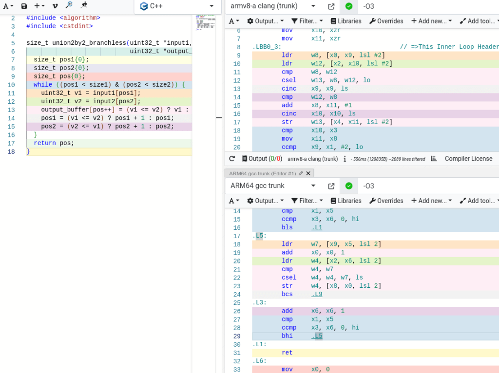

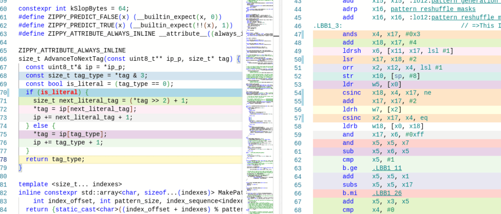
 comparisons on average. We know from Computer Science courses that
 among
among  elements (constant number)
 elements will be to the right of the pivot.
 you know the relation of at most
  elements and all
  elements will still be partitioned to the right. Take
  and you already have quadratic behavior.

 for
for 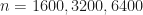 is around
  which are very close to reported numbers. If you read carefully the implementation
 , fall back to heap sort, worst case known algorithm. Even Wikipedia has all good references

 if you can sort
  , condition 5 is a more general upper limit – you should be able to find position of
  in linear amount of comparisons.
 for all input
  ), then it is also optimal towards another. And at this point, theory starts to differ much from reality. Theory found a nice “common” presortedness measure, it’s very complicated and out of scope for this article.
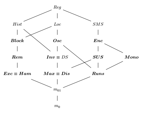
 and it’s an open question whether they have lower complexity). If you want to report some of these measures, you need to sample heavily or add extra
  , we bail out to recursion, otherwise we sort it and don’t go there. That’s really great for almost sorted patterns.
 . Since heapsort’s worst case time complexity is


 -th element) is not necessary. The compiler likely cannot optimize it away.
 is false
 and
and  cannot be both true
 imply
imply 
 and
and  imply
imply  , where


 time. Even though with the existence of
  algorithms (this is for another post), this takes much more time than
  triples and fixed or reported all bugs. Worked like a charm 🙂 . This hasn’t been submitted to LLVM yet as I could not find time to do that properly.


 elements through
  , comparisons, you need to do the following things:
 instructions.


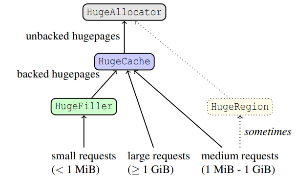
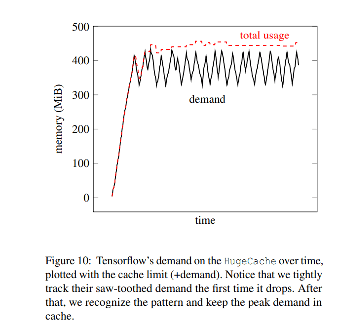

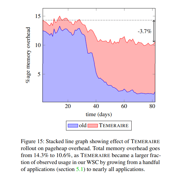

 defines the CRC algorithm and the symbol
  denotes

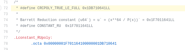
 = 0x1DB710641 This
  only in the final bit: 0x41 vs 0x40. This isn’t coincidental. Calculating
  , with only one ‘on’ bit) by the 33-bit polynomial
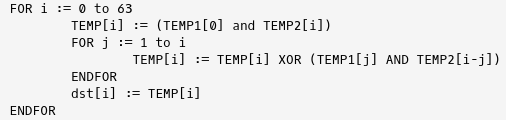
 smallest and sort them. For example, it is widely used in SQL queries when you do
  comparisons and we will look at only one example when it is not the case. Yes, there are a bunch of median algorithms that can be generalized to find the
  comparisons if we pick random pivot. That is because if we define
  is the expected number of comparisons for finding
 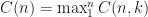 , then during one stage we do
  comparisons and uniformly pick any pivot, then even if we pick the biggest part on each step

 with an obvious induction base, we get
 element of the array or picking pivot from 3 random elements . Or do like
 ![A[0], A[n/2], A[n - 1]](https://s0.wp.com/latex.php?latex=A%5B0%5D%2C+A%5Bn%2F2%5D%2C+A%5Bn+-+1%5D&bg=FFFFFF&fg=181818&s=0&c=20201002) .
.


 of size
  ,
, groups of size 5 and find the median of each group. (For simplicity, we will ignore integrality issues.)
 .
. groups, at least
  of them have at least 3 out of 5 elements that are smaller or equal than
  and we have the reccurence

 which gives us the result
  .
. is at least 1 because we need to partition the array, then finding median out of 5 elements cannot be done in less than 6 comparisons (can be proven by only brute-forcing) and in 6 comparisons it can be done in the following way
![a[1] < a[2], a[4] < a[5]](https://s0.wp.com/latex.php?latex=a%5B1%5D+%3C+a%5B2%5D%2C+a%5B4%5D+%3C+a%5B5%5D&bg=FFFFFF&fg=181818&s=0&c=20201002) , and
, and ![a[1] < a[4]](https://s0.wp.com/latex.php?latex=a%5B1%5D+%3C+a%5B4%5D&bg=FFFFFF&fg=181818&s=0&c=20201002) .
.![a[3] > a[2]](https://s0.wp.com/latex.php?latex=a%5B3%5D+%3E+a%5B2%5D&bg=FFFFFF&fg=181818&s=0&c=20201002) , then the problem is fairly easy. If
, then the problem is fairly easy. If ![a[2] < a[4]](https://s0.wp.com/latex.php?latex=a%5B2%5D+%3C+a%5B4%5D&bg=FFFFFF&fg=181818&s=0&c=20201002) , the median value is the smaller of
, the median value is the smaller of ![a[3]](https://s0.wp.com/latex.php?latex=a%5B3%5D&bg=FFFFFF&fg=181818&s=0&c=20201002) and
and ![a[4]](https://s0.wp.com/latex.php?latex=a%5B4%5D&bg=FFFFFF&fg=181818&s=0&c=20201002) . If not, the median value is the smaller of
. If not, the median value is the smaller of ![a[2]](https://s0.wp.com/latex.php?latex=a%5B2%5D&bg=FFFFFF&fg=181818&s=0&c=20201002) and
and ![a[5]](https://s0.wp.com/latex.php?latex=a%5B5%5D&bg=FFFFFF&fg=181818&s=0&c=20201002) .
.![a[3] < a[2]](https://s0.wp.com/latex.php?latex=a%5B3%5D+%3C+a%5B2%5D&bg=FFFFFF&fg=181818&s=0&c=20201002) . If
. If ![a[3] > a[4]](https://s0.wp.com/latex.php?latex=a%5B3%5D+%3E+a%5B4%5D&bg=FFFFFF&fg=181818&s=0&c=20201002) , then the solution is the smaller of
, then the solution is the smaller of  and it gives us the upper bound
  comparisons which looks like it can be achieved. Some other tricks can be done in place to achieve a bit lower constants like
  (for example, sorting arrays of 5 and comparing less afterwards). In practice, the constant is really big and you can see it from the following demonstration which was even fastened because it took quite a few seconds:
 elements into this heap. C++
  , average
 recursive calls have been made without halving the list size, for some small positive
  QuickSelect steps and if not successful, fallback to HeapSelect algorithm. So, worst case
 elements, use
  elements
 , use
, use 

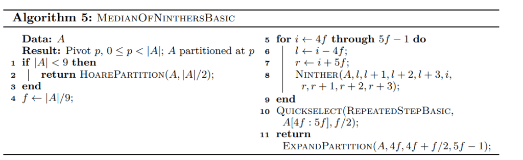
 . MedianOfMedians computes medians of small groups and takes their median to find a pivot approximating the median of the array. In this case, we pursue an order statistic skewed to the left, so instead of the median of each group, we compute its minimum; then, we obtain the pivot by computing the median of those groupwise minima.
 is not chosen arbitrarily because in order to preserve the linearity of the algorithm we need to make sure that while recursing on
  elements we partition more than
  . MedianOfMaxima is done the same way and for
  . The resulting algorithm turns out to be the following

 for all
  which requires only
  comparisons (I am also not going to prove it is minimal but it is). Let’s quickly revise how it works.
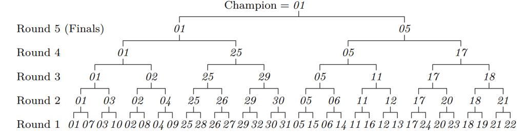

 comparisons for that.
 items. (This takes
  comparisons.) The largest item is greater than
  elements held in reserve, and find the largest element of the resulting
  comparisons because we need to recompute only one path in the tree. Repeat this operation
  comparisons. Assume you need to find top 10 out of millions of long strings and this might be a good solution to this instead of comparing at least

 of size
  from the array.
 and
and  , such that
  (essentially they take
 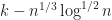 and
and  ). These two elements will be the pivots for the partition and are expected to contain the
  comparisons with probability at least
  (and the constant in the power can be tuned).

 comparisons which is significantly better than all “at least
  which is significantly better.
 and
and  arrays. Benchmark data:

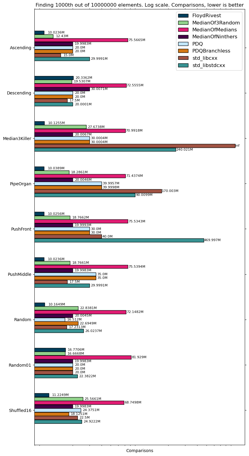

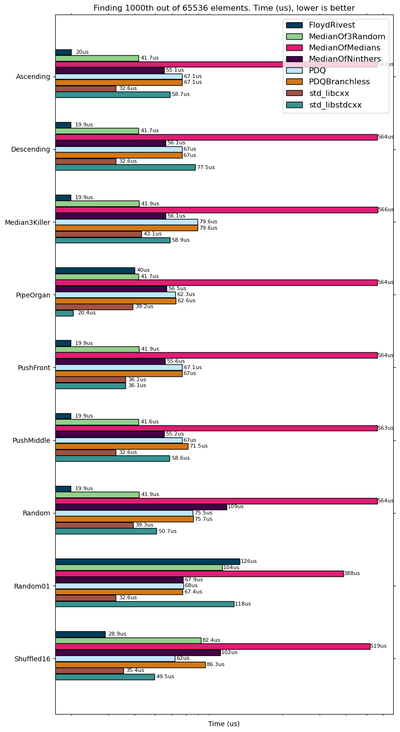


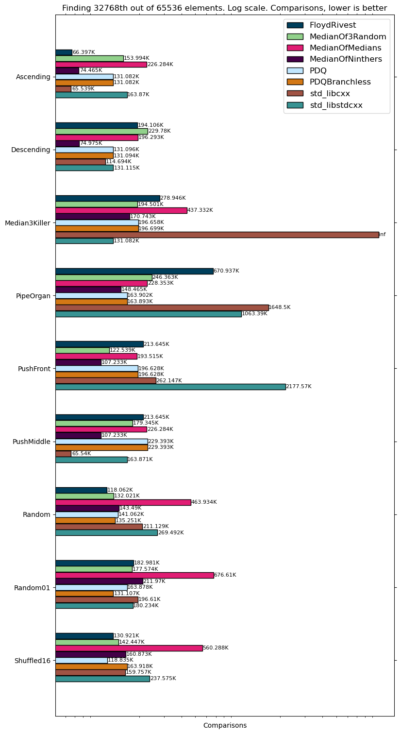
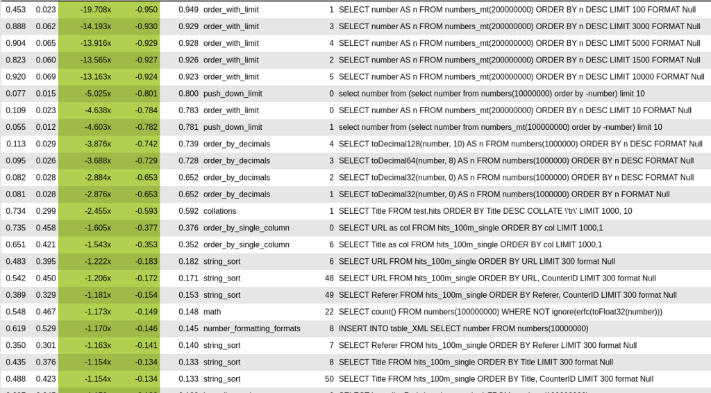
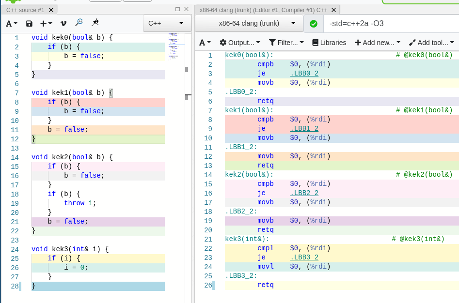


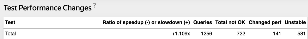
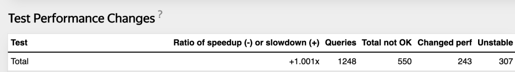
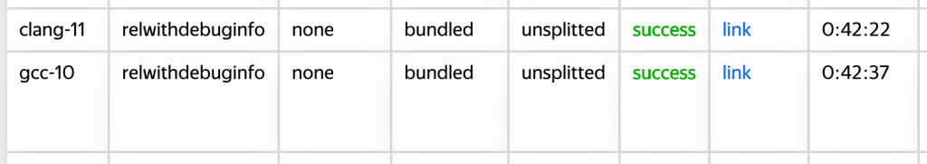


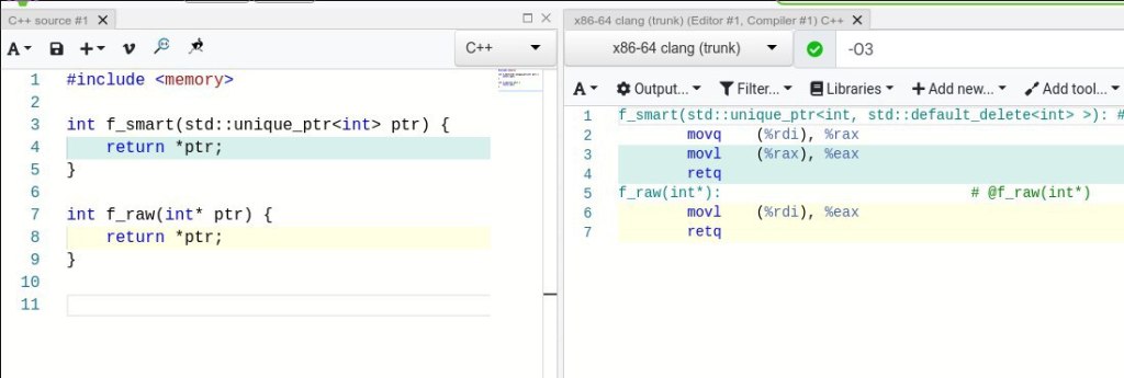


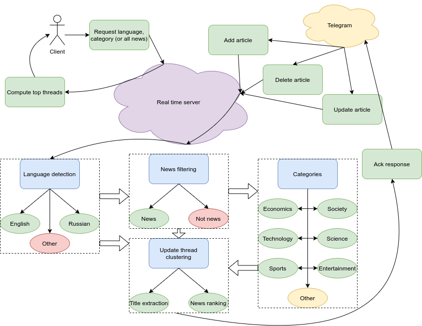


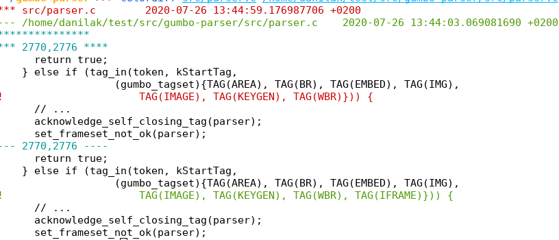

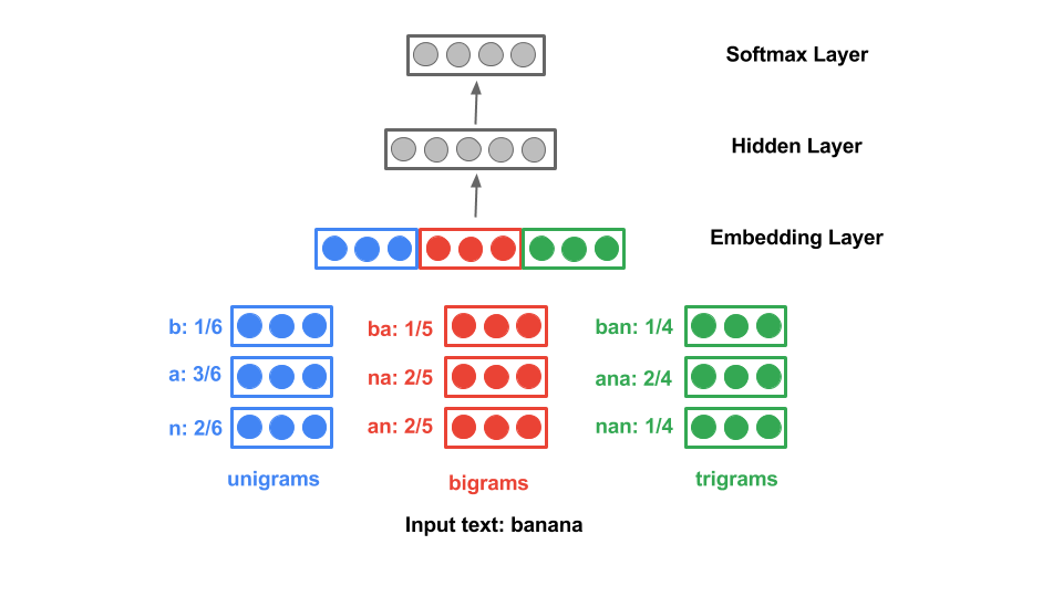


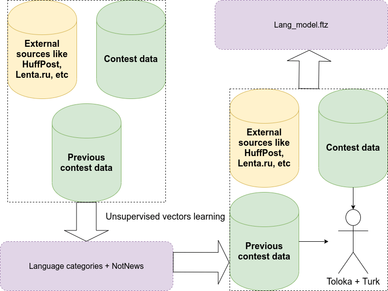

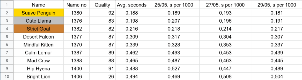
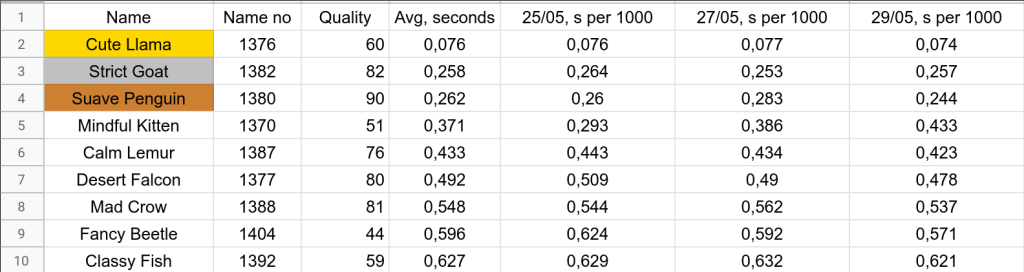


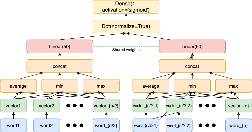
 , in
, in 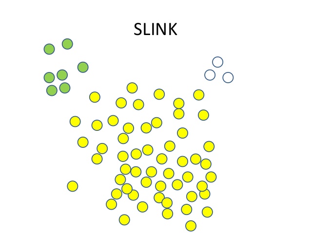


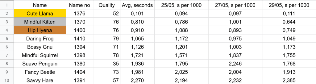


 and the number of shards is $n$) will be around
  and
and  with high probability, so we significantly improving the load balancing between shards. It significantly improves the bound and still allows it to be almost lock free in the shard’s choice. Given the fact there was around 10 QPS in the tests, it is almost optimal.
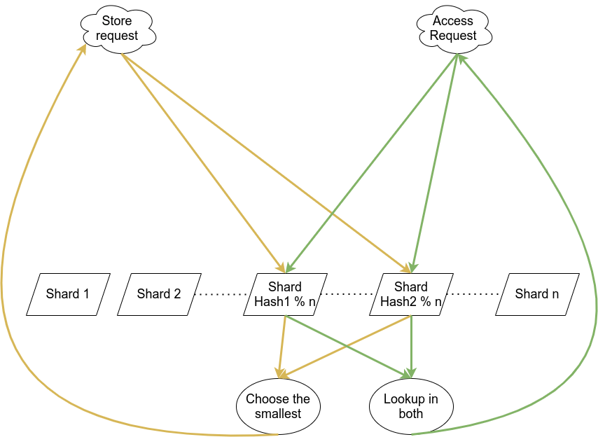
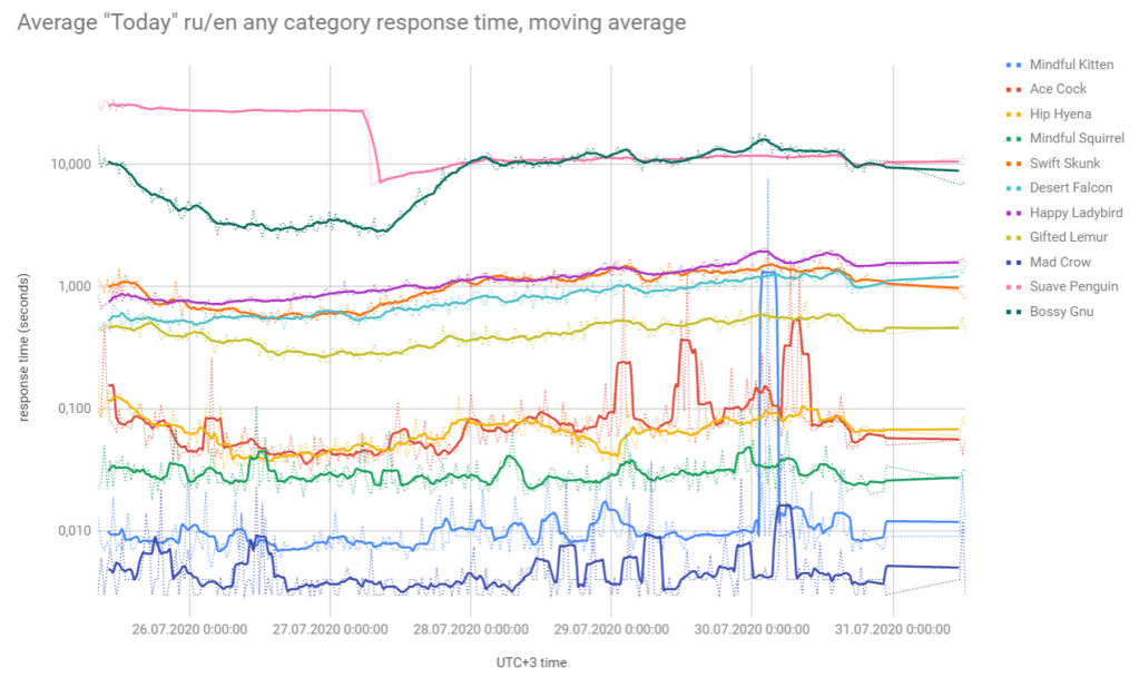

 . In order to preserve this property I decided to do the following:


 threads and was filtering out all the news that are not in line with the request (not the requested category, language, expired or not in the time-frame). Old news will be filtered out, new news remain and are likely relevant, ordering in the cluster preserves the same, title of thread is the title of the most relevant news (to avoid any copyright or misleading issues in the future 🙂 ), thread relevance is recalculated as it is linear in time.
  entities and it can be proven that with some constant probability they will find a collision, i.e. two different objects will have the same hash.

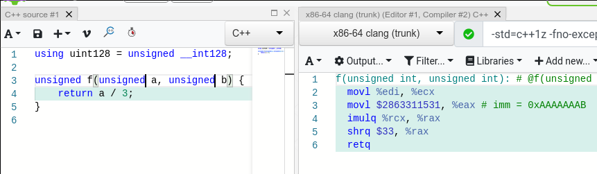
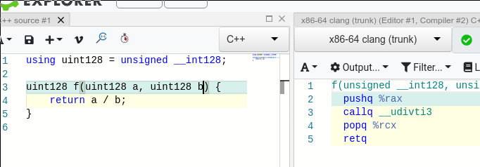


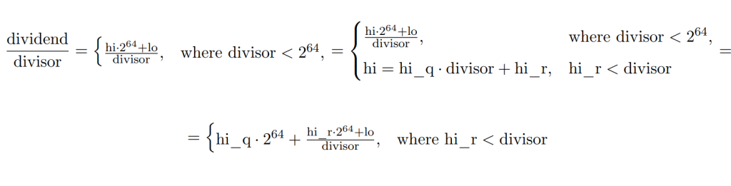
 . We will get something like

 .
. because the maximum value of
  is
is  and minimum value of
  is
is  . Now let’s show that
 .
. .
.  is the largest when the remainder in the numerator is as large as possible, it can be up to
  . Because of the definition of
  . The smallest value of
  in the denominator is
  . That’s why
 . As n iterates from 0 to 63, we can conclude that
  . So we got either the correct value, either the correct plus one. Everything else in the algorithms is just a correction of which result to choose.
 in the screenshot below and it showed some inconsistent results which I don’t understand for now.
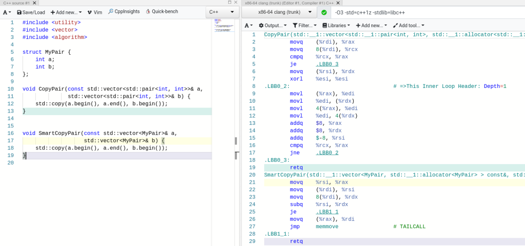
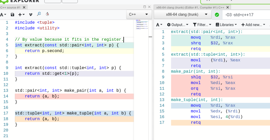
 books and
  libraries. Books somehow assigned to libraries, one book can be in many libraries. Each book has a score
  , each library has install time
  and daily throughput
  (maximum number of books shipped per day). We can only choose one library, wait for its install time, then choose another and so on but all libraries push their books at the same time and when they are ready. We need to maximize the score of all books given
  days. Look at the example if you did not get the statement.
 days to ship books.
 where
where  represents the vector of variables (to be determined),
  are vectors of (known) coefficients,
  is the matrix transpose.
 ). The only requirement — the relations must be linear.
 variables and conditions. Or at least they can find some solutions that are quite good. We will talk about solvers a bit later.
 vector which sometimes makes the problem much better. Solvers are less happy about the integer programming — it is NP-complete partially because
  variables. For more only luck and the variety of the solvers can help. Though, you can do something good even with that big amount of variables about which we will talk a bit later.
 means OR,
  means AND)
 variables and clauses (clause is a disjunction of variables). Also, there is a really good
  with the squares
  is a NP-complete problem,
  . Number
  is kind of important: it is shown by many different papers that this is likely a transition phase number for random 3SATs (so, if the ratio is bigger than that, 3SAT is easy to solve, if less, also easy but if it is around, 3SAT becomes complex). Random 3SAT does embrace a phase transition phenomenon! That’s kind of a funny fact and showed even within some physics laws
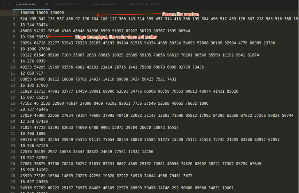
 . (maximizing the weighted sum of covered books).
 ; (the installation time of the selected libraries cannot exceed
  ; (if a book is chosen, i.e.
  then at least one library where this book presents
  is selected).
 ; (if
; (if  then book
  is chosen)
 (if
(if  then library
  is selected for the cover).
 approximation. And this solution brings us ~5,689,000 points. After that, I moved it to a SCIP solver as a hint and after 20 seconds it said it found the optimum in 5,690,556 points and that’s it. Dataset is cracked.
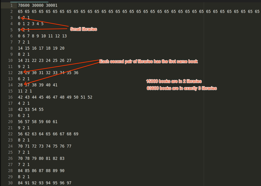
 which means that it is likely common to random 3SAT with a transition phase. So, basically I split 30000 libraries in pairs, each pair is a variable in 3SAT, if you choose the first one, this is true, otherwise false, other books in the libraries are the clauses numbers, in the first element there are the clauses that contain the variable, in the second the negation of this variable. Then I created a 3SAT with 15000 variables which the world believes it is hard to solve.